PVT
The PVT block is the last one in the GNSS-SDR flow graph. Hence, it acts as a signal sink, since the stream of data flowing along the receiver ends here.
The role of a PVT block is to compute navigation solutions and deliver information in adequate formats for further processing or data representation.
It follows a description of the available positioning algorithms and their parameters, the available output formats, and the description of the configuration options for this block.
Positioning modes
The positioning problem is generally stated as
\[\begin{equation} \mathbf{y} = \mathbf{h}(\mathbf{x}) + \mathbf{n}~, \end{equation}\]where \(\mathbf{y}\) is the measurement vector (that is, the observables
obtained from the GNSS signals of a set of \(m\) satellites), \(\mathbf{x}\)
is the state vector to be estimated (at least, the position of the receiver’s
antenna and the time), \(\mathbf{h}(\cdot)\) is the function that relates
states with measurements, and \(\mathbf{n}\) models measurement noise.
Depending on the models, assumptions, available measurements, and the
availability of a priori or externally-provided information, many positioning
strategies and algorithms can be devised. It follows a description of the
positioning modes available at the RTKLIB_PVT
implementation, mostly extracted from the excellent RTKLIB
manual.
Single Point Positioning
The default positioning mode is PVT.positioning_mode=Single. In this mode, the
vector of unknown states is defined as:
where \(\mathbf{r}_r\) is the receiver’s antenna position in an earth-centered, earth-fixed (ECEF) coordinate system (in meters), \(c\) is the speed of light, and \(dt_r\) is the receiver clock bias (in seconds).
The measurement vector is defi
\[\begin{equation} \mathbf{y} = \left(P_r^{(1)}, P_r^{(2)}, P_r^{(3)}, ..., P_r^{(m)} \right)^T~. \end{equation}\]As described in the Observables block, for a signal from satellite \(s\) in the i-th band, the pseudorange measurement \(P_{r,i}^{(s)}\) can be expressed as:
\[\begin{equation} P_{r,i}^{(s)} = \rho_r^{(s)} + c\left(dt_r(t_r) - dT^{(s)}(t^{(s)}) \right) + I_{r,i}^{(s)} + T_r^{(s)} + \epsilon_P~. \end{equation}\]In the current implementation, if the receiver obtains pseudorange measurements from the same satellite in different frequency bands, only measurements in the L1 band are used.
Hence, the equation that relates pseudorange measurements to the vector of unknown states can be written as:
\[\begin{equation} \mathbf{h}(\mathbf{x}) = \left( \begin{array}{c} \rho_{r}^{(1)} + c \cdot dt_r - c \cdot dT^{(1)} + I_{r}^{(1)} + T_{r}^{(1)} \\ \rho_{r}^{(2)} + c \cdot dt_r - c \cdot dT^{(2)} + I_{r}^{(2)} + T_{r}^{(2)} \\ \rho_{r}^{(3)} + c \cdot dt_r - c \cdot dT^{(3)} + I_{r}^{(3)} + T_{r}^{(3)} \\ \vdots \\ \rho_{r}^{(m)} + c \cdot dt_r - c \cdot dT^{(m)} + I_{r}^{(m)} + T_{r}^{(m)} \end{array} \right)~. \end{equation}\]The geometric range \(\rho_r^{(s)}\) is defined as the physical distance between the satellite antenna phase center position and the receiver antenna phase center position in the inertial coordinates. For the expression in the ECEF coordinates, the earth rotation effect has to be incorporated. This is known as the Sagnac effect1, and it can be approximated by:
\(\begin{equation} \rho_{r}^{(s)} \approx \left\| \mathbf{r}_r(t_r) - \mathbf{r}^{(s)}(t^{(s)}) \right\| + {\definecolor{dark-orange}{RGB}{255,165,0} \color{dark-orange} \frac{\omega_e}{c}\left(x^{(s)}y_r - y^{(s)}x_r \right)}~, \end{equation}\) where \(\omega_e\) is the Earth rotation angle velocity (in rad/s).
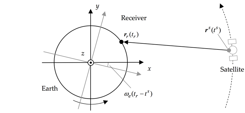 Geometric range and Earth rotation correction 2
Equation \(\mathbf{h}(\mathbf{x})\) is clearly nonlinear due to the presence of the Euclidean norm operator \(\left\| \cdot \right\|\). However, this term can be extended by using Taylor series around an initial parameter vector \(\mathbf{x}_0\) as \(\mathbf{h}(\mathbf{x}) = \mathbf{h}(\mathbf{x}_0) + \mathbf{H}(\mathbf{x}-\mathbf{x}_0) + ...\), where \(\mathbf{H} = \frac{\partial \mathbf{h}(\mathbf{x})}{\partial \mathbf{x}} \bigg\rvert_{\mathbf{x} = \mathbf{x}_{0} }\) is a partial derivatives matrix of \(\mathbf{h}(\mathbf{x})\) with respect to \(\mathbf{x}\) at \(\mathbf{x} = \mathbf{x}_{0}\). Assuming that the initial parameters are adequately near the true values and the second and further terms of the Taylor series can be neglected, equation \(\mathbf{y} = \mathbf{h}(\mathbf{x}) + \mathbf{n}\) can be approximated by \(\mathbf{y} \approx \mathbf{h}(\mathbf{x}_0) + \mathbf{H}(\mathbf{x}-\mathbf{x}_0) + \mathbf{n}\), and then we can obtain the following linear equation:
\[\begin{equation} \mathbf{y} - \mathbf{h}(\mathbf{x}_0) = \mathbf{H}(\mathbf{x}-\mathbf{x}_0) + \mathbf{n}~, \end{equation}\]which can be solved by a standard iterative weighted least squares method.
Matrix \(\mathbf{H}\) can be written as:
\[\begin{equation} \label{eq:H-single} \mathbf{H} = \left( \begin{array}{cc} - {\mathbf{e}_{r}^{(1)}}^T & 1 \\ -{\mathbf{e}_{r}^{(2)}}^T & 1 \\ -{\mathbf{e}_{r}^{(3)}}^T & 1 \\ \vdots & \vdots \\ -{\mathbf{e}_{r}^{(m)}}^T & 1 \end{array} \right), \quad \text{where } \mathbf{e}_r^{(s)} = \frac{\mathbf{r}^{(s)}(t^{(s)}) - \mathbf{r}_r(t_r) }{\left\| \mathbf{r}^{(s)}(t^{(s)}) - \mathbf{r}_r(t_r) \right\|} \end{equation}\]and the weighted least squares estimator (LSE) of the unknown state vector is obtained as:
For the initial parameter vector \(\mathbf{x}_0\) for the iterated weighted
LSE, just all \(0\) are used for the first epoch of the single point
positioning. Once a solution obtained, the position is used for the next epoch
initial receiver position. For the weight matrix \(\mathbf{W}\), the
RTKLIB_PVT implementation uses:
where:
-
\(F^{(s)}\) is the satellite system error factor. This parameter is set to \(F^{(s)} = 1\) for GPS and Galileo.
-
\(R_r\) is the code/carrier‐phase error ratio. This value is set by default to \(R_r = 100\), and can be configured with the
PVT.code_phase_error_ratio_l1option. -
\(a_{\sigma}, b_{\sigma}\) is the carrier‐phase error factor \(a\) and \(b\) (in m). They are set by default to \(a_{\sigma} = b_{\sigma} = 0.003\) m, and can be configured with the
PVT.carrier_phase_error_factor_aandPVT.carrier_phase_error_factor_boptions, respectively. -
\(El_r^{(s)}\) is the elevation angle of satellite direction (in rad).
-
\(\sigma_{bclock,s}\) is the standard deviation of the broadcast ephemeris and clock error (in m). This parameter is estimated internally from URA (User Range Accuracy) or or similar indicators.
-
\(\sigma_{ion,s}\) is the standard deviation of ionosphere correction model error (in m). This parameter is set to \(\sigma_{ion} = 5\) m by default (
PVT.iono_model=OFF) and \(\sigma_{ion} = 0.5 \cdot I_{r,i}^{(s)}\) m when the optionPVT.iono_model=Broadcastis set in the configuration file. -
\(\sigma_{trop,s}\) is the standard deviation of troposphere correction model error (in m). This parameter is set to \(\sigma_{trop} = 3\) m by default (
PVT.trop_model=OFF) and \(\sigma_{trop} = 0.3 / \left(\sin(El_r^{(s)}) + 0.1\right)\) m when the optionPVT.trop_model=Saastamoinen,PVT.trop_model=Estimate_ZTDorPVT.trop_model=Estimate_ZTD_Gradis set in the configuration file. -
\(\sigma_{cbias}\) is the standard deviation of code bias error (in m). This parameter is set to \(\sigma_{cbias} = 0.3\) m.
In addition, two optional terms can extend this
error model. These options are only present in the
next branch of the upstream repository, and will be included in the next
GNSS-SDR stable release.
-
An SNR-dependent term, activated when
\[e_{\sigma}^2 \cdot 10^{~0.1 \cdot \max \left( \text{SNR}_{\text{max}} - C/N_0^{(s)},~ 0 \right)}~,\]PVT.error_factor_snris set to a positive value \(e_{\sigma}\) (in m; ta recommended value is \(0.005\) m), which adds to the variance a termwhere \(C/N_0^{(s)}\) is the carrier-to-noise density ratio reported by the tracking loop for satellite \(s\), and \(\text{SNR}_{\text{max}}\) is a reference value (in dB-Hz) above which no penalty is applied, configurable with
PVT.error_snr_max(it defaults to \(52\) dB-Hz). It defaults to \(0.0\) (disabled), preserving the elevation-only error model. -
A receiver-reported standard deviation term, activated when
PVT.error_factor_rcv_stdis set to a positive value, which weights each observation with the pseudorange / carrier-phase standard deviations reported in the observation structure (fields ready to be populated from the tracking-loop variance estimates). It defaults to \(0.0\) (disabled).
By default, the receiver clock bias estimated in single point positioning is
assumed to be common to all GPS-like signals, including QZSS. Setting
PVT.estimate_qzss_isb=true adds a separate QZS-GPS inter-system bias to the
vector of unknowns. The estimated offset is
reported in the RTKLIB solution structure (sol.dtr[4]). Since the extra
unknown requires one more satellite in mixed GPS + QZSS epochs, which degrades
availability under limited sky visibility, this option defaults to false and
should only be enabled in open-sky scenarios with six or more satellites in
view. This option is only present in the next
branch of the upstream repository, and will be included in the next GNSS-SDR
stable release.
The estimated receiver clock bias \(dt_r\) is not explicitly output, but incorporated in the solution time‐tag. That means the solution time‐tag indicates not the receiver time‐tag but the true signal reception time measured in GPS Time.
Solution validation
The estimated receiver positions described in (\(\ref{eq:lse}\)) might include
invalid solutions due to unmodeled measurement errors. To test whether the
solution is valid or not, and to reject the invalid solutions, the RTKLIB_PVT
applies the following validation tests after obtaining the receiver’s position
estimate:
1) Residuals Test
Defining the residuals vector \(\boldsymbol{\nu} = \left( \nu_1, \nu_2, \nu_3, ..., \nu_m \right)^T\) with:
\[\nu_s = \frac{P_r^{(s)} - \left( \hat{\rho}_r^{(s)} + c \hat{dt}_r - c \cdot dT^{(s)} + I_r^{(s)} + T_r^{(s)} \right)}{\sigma_s}~,\]the residuals test is defined as:
\[\frac{\boldsymbol{\nu}^T \boldsymbol{\nu}}{m-n-1} < \chi_{\alpha}^2 (m-n-1)\]where \(n\) is the number of estimated parameters, \(m\) is the number of measurements, \(\chi_{\alpha}^2(n)\) is the chi‐square distribution of degree of freedom \(n\), and with a significance level of \(\alpha=0.001\) (that is, \(prob > 0.001\)).
2) GDOP Test
The Geometric Dilution of Precision, defined as \(\text{GDOP} = \sqrt{\sigma_{r_{x}}^2 + \sigma_{r_{y}}^2 + \sigma_{r_{z}}^2 + \sigma_{c \cdot dt}^2 }\), must be better (that is, lower) than a certain threshold:
\[\text{GDOP} < \text{GDOP}_{\text{threshold}}\]The threshold value is set by default to \(\text{GDOP}_{\text{threshold}} =
30\), and it can be configured via the option PVT.threshold_reject_GDOP in the
configuration file.
If any of the validation fails, the solution is rejected as an outlier (that is, no solution is provided).
Receiver Autonomous Integrity Monitoring (RAIM)
In addition to the solution validation described above, RAIM (receiver
autonomous integrity monitoring) FDE (fault detection and exclusion) function
can be activated. If the chi-squared test described above fails and the option
PVT.raim_fde is set to \(1\), the implementation retries the estimation by
excluding one by one of the visible satellites. After all of the retries, the
estimated receiver position with the minimum normalized squared residuals
\(\boldsymbol{\nu}^T \boldsymbol{\nu}\) is selected as the final solution. In
such a scheme, an invalid measurement, which might be due to satellite
malfunction, receiver fault, or large multipath, is excluded as an outlier. Note
that this feature is not effective with two or more invalid measurements. It
also needs two redundant visible satellites, which means at least 6 visible
satellites are necessary to obtain the final solution.
Precise Point Positioning
When the PVT.positioning_mode option is set to PPP_Static or PPP_Kinematic
in the configuration file, a Precise Point Positioning algorithm is used to
solve the positioning problem. In this positioning mode, the state vector to be
estimated is defined as:
where \(Z_r\) is ZTD (zenith total delay), \(G_{N_r}\) and \(G_{E_r}\) are the north and east components of tropospheric gradients (see the tropospheric model below) and \(\mathbf{B}_{LC} = \left( B_{r,LC}^{(1)}, B_{r,LC}^{(2)}, B_{r,LC}^{(3)}, ..., B_{r,LC}^{(m)} \right)^T\) is the ionosphere‐free linear combination of zero‐differenced carrier‐phase biases (in m), defined below in Equation (\(\ref{eq:bias-lc}\)).
The Precise Point Positioning measurement model is based on the fact that, according to the phase and code ionospheric refraction, the first order ionospheric effects on code and carrier-phase measurements depend (99.9 %) on the inverse of squared signal frequency \(f_i\). Thence, dual-frequency receivers can eliminate their effect through a linear combination of pseudorange \(P_{r,i}^{(s)}\) and phase-range \(\Phi_{r,i}^{(s)}\) measurements (where the definitions at Observables apply):
\[P_{r,LC}^{(s)} = C_i P_{r,i}^{(s)} + C_j P_{r,j}^{(s)}\] \[\Phi_{r,LC}^{(s)} = C_i \Phi_{r,i}^{(s)} + C_j \Phi_{r,j}^{(s)}\]with \(C_i = \frac{f_i^2}{f_i^2 - f_j^2}\) and \(C_j = \frac{-f_j^2}{f_i^2 - f_j^2}\), where \(f_i\) and \(f_j\) are the frequencies (in Hz) of \(L_i\) and \(L_j\) measurements. Explicitly:
\[\begin{equation} P_{r,LC}^{(s)} = \rho_{r}^{(s)} + c\left(dt_r - dT^{(s)}\right) + T_{r}^{(s)} + \epsilon_P \end{equation}\] \[\begin{equation} \Phi_{r,LC}^{(s)} = \rho_{r}^{(s)} + c\left(dt_r - dT^{(s)}\right) + T_{r}^{(s)} + B_{r,LC}^{(s)} + d\Phi_{r,LC}^{(s)} + \epsilon_{\Phi} \end{equation}\]with
\[\begin{equation} \label{eq:bias-lc} B_{r,LC}^{(s)} = C_i \left( \phi_{r,0,i} - \phi_{0,i}^{(s)} + N_{r,i}^{(s)} \right) + C_j \left( \phi_{r,0,j} - \phi_{0,j}^{(s)} + N_{r,j}^{(s)} \right) \end{equation}\] \[\begin{equation} \begin{array}{ccl} d\Phi_{r,LC}^{(s)} & = & - \left( C_i \mathbf{d}_{r,pco,i} + C_j C_i \mathbf{d}_{r,pco,i} \right)^T \mathbf{e}_{r,enu}^{(s)} + \\ {} & {} & + \left( \mathbf{E}^{(s)} \left( C_i \mathbf{d}_{pco,i}^{(s)} + C_j\mathbf{d}_{pco,j}^{(s)} \right) \right)^T \mathbf{e}_r^{(s)} + \\ {} & {} & + \left( C_i d_{r,pcv,i}(El_{r}^{(s)}) + C_j d_{r,pcv,j}(El_{r}^{(s)}) \right) + \\ {} & {} & + \left( d_{pcv,i}^{(s)}(\theta) + d_{pcv,j}^{(s)}(\theta)\right) + \\ {} & {} & - \mathbf{d}_{r,disp}^T \mathbf{e}_{r,enu}^{(s)} +\left( C_i\lambda_i + C_j \lambda_j \right) \phi_{pw} \end{array} \end{equation}\]In the current implementation, satellites and receiver antennas offset and
variation are not applied, so \(\mathbf{d}_{r,pco,i} = \mathbf{d}_{pco,i}^{(s)} =
\mathbf{0}\) and \(d_{r,pcv,i} = d_{pcv,j}^{(s)} = 0\). The correction terms
for the Earth tide3 \(\mathbf{d}_{r,disp}\) and the phase windup
effect4 \(\phi_{pw}\) are deactivated by default, and can be
activated through the PVT.earth_tide and PVT.phwindup options, respectively.
The measurement vector is then defined as:
\[\begin{equation} \mathbf{y} = \left( \boldsymbol{\Phi}_{LC}^T, \mathbf{P}_{LC}^T \right)^T~, \end{equation}\]where \(\boldsymbol{\Phi}_{LC} = \left(\Phi_{r,LC}^{(1)}, \Phi_{r,LC}^{(2)}, \Phi_{r,LC}^{(3)}, ..., \Phi_{r,LC}^{(m)} \right)^T\) and \(\mathbf{P}_{LC} = \left( P_{r,LC}^{(1)}, P_{r,LC}^{(2)}, P_{r,LC}^{(3)}, ..., P_{r,LC}^{(m)} \right)^T\).
In the current implementation, if the receiver obtains pseudorange measurements from the same satellite in different frequency bands, only measurements in the L1 band are used.
The equation \(\mathbf{h}(\mathbf{x})\) that relates measurements and states is:
\[\begin{equation} \mathbf{h}(\mathbf{x}) = \left( \mathbf{h}_{\Phi}^T, \mathbf{h}_{P}^T \right)^T~, \end{equation}\]where:
\[\mathbf{h}_{\Phi} = \left( \begin{array}{c} \rho_{r}^{(1)} + c(dt_r - dT^{(1)}) + T_{r}^{(1)} + B_{r,LC}^{(1)} + d\Phi_{r,LC}^{(1)} \\ \rho_{r}^{(2)} + c(dt_r - dT^{(2)}) + T_{r}^{(2)} + B_{r,LC}^{(2)} + d\Phi_{r,LC}^{(2)} \\ \rho_{r}^{(3)} + c(dt_r - dT^{(3)}) + T_{r}^{(3)} + B_{r,LC}^{(3)} + d\Phi_{r,LC}^{(3)} \\ \vdots \\ \rho_{r}^{(m)} + c(dt_r - dT^{(m)}) + T_{r}^{(m)} + B_{r,LC}^{(m)} + d\Phi_{r,LC}^{(m)} \end{array}\right)~,\] \[\mathbf{h}_{P} = \left( \begin{array}{c} \rho_{r}^{(1)} + c(dt_r - dT^{(1)}) + T_{r}^{(1)} \\ \rho_{r}^{(2)} + c(dt_r - dT^{(2)}) + T_{r}^{(2)} \\ \rho_{r}^{(3)} + c(dt_r - dT^{(3)}) + T_{r}^{(3)} \\ \vdots \\ \rho_{r}^{(m)} + c(dt_r - dT^{(m)}) + T_{r}^{(m)} \end{array}\right)~.\]This is again a nonlinear equation that could be solved with the iterative weighted least squares estimator as in the case of the Single Point Positioning case. However, here we want to incorporate some a priori information, such as a basic dynamic model for the receiver, and some statistical knowledge about the status of the troposphere. The Extended Kalman Filter offers a suitable framework for that.
The partial derivatives matrix \(\mathbf{H} = \frac{\partial \mathbf{h}(\mathbf{x})}{\partial \mathbf{x}} \bigg\rvert_{\mathbf{x} = \mathbf{x}_{0} }\) can be written as:
\[\begin{equation} \mathbf{H}(\mathbf{x}) = \left(\begin{array}{ccccc} - \mathbf{DE} & \mathbf{0} & \mathbf{1} & \mathbf{DM}_T && \mathbf{I} \\ -\mathbf{DE} & \mathbf{0} & \mathbf{1} & \mathbf{DM}_T && \mathbf{0} \end{array} \right)~, \end{equation}\]where \(\mathbf{D} = \left( \begin{array}{ccccc} 1 & -1 & 0 & \cdots & 0 \\ 1 & 0 & -1 & \cdots & 0 \\ \vdots & \vdots & \vdots & \ddots & \vdots \\ 1 & 0 & 0 & \cdots & -1 \end{array} \right)\) is known as the single‐differencing matrix, \(\mathbf{E} = \left( \mathbf{e}_{r}^{(1)}, \mathbf{e}_{r}^{(2)}, \mathbf{e}_{r}^{(3)}, ..., \mathbf{e}_{r}^{(m)} \right)^T\) with \(\mathbf{e}_{r}^{(s)}\) defined as in equation (\(\ref{eq:H-single}\)), and
\(\scriptstyle \begin{equation} \!\!\!\!\!\!\!\!\!\!\! \mathbf{M}_T \; = \; \left( \begin{array}{ccc} m_{WG,r}^{(1)} \left( El_r^{(1)} \right) & m_{W,r}^{(1)} \left( El_r^{(1)} \right) \cot \left( El_r^{(1)} \right) \cos \left( Az_r^{(1)} \right) & m_{W,r}^{(1)} \left( El_r^{(1)} \right) \cot \left( El_r^{(1)} \right) \sin \left( Az_r^{(1)} \right) \\ m_{WG,r}^{(2)} \left( El_r^{(2)} \right) & m_{W,r}^{(2)} \left( El_r^{(2)} \right) \cot \left( El_r^{(2)} \right) \cos \left( Az_r^{(2)} \right) & m_{W,r}^{(2)} \left( El_r^{(2)} \right) \cot \left( El_r^{(2)} \right) \sin \left( Az_r^{(2)} \right) \\ m_{WG,r}^{(3)} \left( El_r^{(3)} \right) & m_{W,r}^{(3)} \left( El_r^{(3)} \right) \cot \left( El_r^{(3)} \right) \cos \left( Az_r^{(3)} \right) & m_{W,r}^{(3)} \left( El_r^{(3)} \right) \cot \left( El_r^{(3)} \right) \sin \left( Az_r^{(3)} \right) \\ \vdots \\ m_{WG,r}^{(m)} \left( El_r^{(m)} \right) & m_{W,r}^{(m)} \left( El_r^{(m)} \right) \cot \left( El_r^{(m)} \right) \cos \left( Az_r^{(m)} \right) & m_{W,r}^{(m)} \left( El_r^{(m)} \right) \cot \left( El_r^{(m)} \right) \sin \left( Az_r^{(m)} \right) \end{array} \right) \end{equation}\) is a matrix related to the tropospheric model (see below).
With all those definitions, the Precise Point Positioning solution is computed as follows:
- Time update (prediction):
- Measurement update (estimation):
The transition matrix \(\mathbf{F}_k\) models the receiver movement:
- If
PVT.positioning_mode=PPP_Static:
- If
PVT.positioning_mode=PPP_Kinematic:
where \(\Delta_k = t_{k+1} - t_k\) is the time between GNSS measurements, in s.
The dynamics model noise covariance matrix \(\mathbf{Q}_k\) is set to:
\[\begin{equation} \mathbf{Q}_k = \left(\begin{array}{ccccc} \mathbf{Q}_{r} & {} & {} & {} & {} \\ {} & \mathbf{Q}_{v} & {} & {} & {} \\ {} & {} & \sigma_{c \cdot dt_{r}}^2 & {} & {} \\ {} & {} & {} & \mathbf{Q}_{T} & {} \\ {} & {} & {} & {} & \sigma_{bias}^2 \Delta_k \mathbf{I}_{m\times m} \end{array} \right) \end{equation}\]with:
- \(\mathbf{Q}_r = \mathbf{E}_r^T \text{diag} \left( \sigma_{re}^2 ,
\sigma_{rn}^2 , \sigma_{ru}^2 \right) \mathbf{E}_r\), where \(\mathbf{E}_r\) is the coordinates rotation matrix from ECEF to local
coordinates at the receiver antenna position (defined below), and
\(\sigma_{re}\), \(\sigma_{rn}\) and \(\sigma_{ru}\) are the standard
deviations of east, north, and up components of the receiver position model
noises (in m).
- If the positioning mode is set to
PVT.positioning_mode=PPP_Static, these values are initialized to \(\sigma_{re} = \sigma_{rn} = \sigma_{ru} = 100\) m in the first epoch and then set to \(0\) in the following time updates. - If the positioning mode is set to
PVT.positioning_mode=PPP_Kinematic, these values are set to \(\sigma_{re} = \sigma_{rn} = \sigma_{ru} = 100\) m for all time updates.
- If the positioning mode is set to
- \(\mathbf{Q}_v = \mathbf{E}_r^T \text{diag} \left( \sigma_{ve}^2 \Delta_k , \sigma_{vn}^2 \Delta_k, \sigma_{vu}^2 \Delta_k \right) \mathbf{E}_r\), where \(\sigma_{ve}\), \(\sigma_{vn}\) and \(\sigma_{vu}\) are the standard deviations of east, north, and up components of the receiver velocity model noises (in m/s/\(\sqrt{s}\)). In the current implementation, those parameters are set to \(\sigma_{ve} = \sigma_{vn} = \sigma_{vu} = 0\).
- \(\sigma_{c \cdot dt_{r}}\) is the standard deviation of the receiver clock offset (in m). This value is set to \(\sigma_{c \cdot dt_{r}} = 100\) m.
- \(\mathbf{Q}_{T} = \text{diag} \left( \sigma_{Z}^2 \Delta_k,
\sigma_{G_{N}}^2 \Delta_k, \sigma_{G_{E}}^2 \Delta_k \right)\) is the noise
covariance matrix of the troposphere terms. These values are set to \(\sigma_{Z} = 0.0001\), and \(\sigma_{G_{N}} = \sigma_{G_{E}}\) are
initialized to \(\sigma_{G_{N}} = \sigma_{G_{E}} = 0.001\) m/\(\sqrt{s}\)
in the first epoch and then set to \(\sigma_{G_{N}} = \sigma_{G_{E}} = 0.1
\cdot \sigma_{Z}\) in the following time updates. The default value of \(\sigma_{Z} = 0.0001\) m/\(\sqrt{s}\) can be configured with the
PVT.sigma_tropoption. - \(\sigma_{bias}\) is the standard deviation of the ionosphere-free
carrier-phase bias measurements, in m/\(\sqrt{s}\). This value is
initialized at the first epoch and after a cycle slip to \(\sigma_{bias} =
100\) m/\(\sqrt{s}\), and then is set to a default value of \(\sigma_{bias} = 0.0001\) m/\(\sqrt{s}\) in the following time updates.
This value and can be configured with the option
PVT.sigma_bias. - \(\mathbf{E}_r = \left( \begin{array}{ccc} - \sin(\theta_r) & \cos (\theta_r) & 0 \\ -\sin (\psi_r) \cos(\theta_r) & - \sin (\psi_r)\sin(\theta_r) & \cos (\psi_r) \\ \cos(\psi_r)\cos(\theta_r) & \cos(\psi_r)\sin(\theta_r) & \sin(\psi_r)\end{array} \right)\) is the rotation matrix of the ECEF coordinates to the local coordinates, where \(\psi_r\) and \(\theta_r\) are the geodetic latitude and the longitude of the receiver position.
The measurement model noise covariance matrix \(\mathbf{R}_k\) is defined as:
\[\begin{equation} \mathbf{R} = \left( \begin{array}{cc} \mathbf{R}_{\Phi,LC} & \mathbf{0} \\ \mathbf{0} & \mathbf{R}_{P,LC} \end{array}\right)~, \end{equation}\]where:
\[\mathbf{R}_{\Phi,LC} = \text{diag} \left( {\sigma_{\Phi,1}^{(1)}}^2, {\sigma_{\Phi,1}^{(2)}}^2, {\sigma_{\Phi,1}^{(3)}}^2, ..., {\sigma_{\Phi,1}^{(m)}}^2 \right)~,\] \[\mathbf{R}_{P,LC} = \text{diag} \left( {\sigma_{P,1}^{(1)}}^2, {\sigma_{P,1}^{(2)}}^2, {\sigma_{P,1}^{(3)}}^2, ..., {\sigma_{P,1}^{(m)}}^2 \right)~,\]in which \(\sigma_{\Phi,1}^{(s)}\) is the standard deviation of L1 phase‐range measurement error (in m), and \(\sigma_{P,1}^{(s)}\) is the standard deviation of L1 pseudorange measurement error (in m). These quantities are estimated as:
- \({\sigma_{\Phi,1}^{(s)}}^2 = a_{\sigma}^2 + \frac{b_{\sigma}^2}{\sin(E_r^{(s)})^2} + \sigma_{ion,s}^2 + \sigma_{bclock}^2 + \sigma_{trop,s}^2\), where:
- \(a_{\sigma} = 0.003\) and \(b_{\sigma} = 0.003\) are the carrier
phase error factors (configurable via
PVT.carrier_phase_error_factor_aandPVT.carrier_phase_error_factor_b), - \(\sigma_{ion,s}\) is the standard deviation of ionosphere correction
model error (in m). This parameter is set to \(\sigma_{ion} = 5\) m by
default (
PVT.iono_model=OFF) and \(\sigma_{ion} = 0.5 \cdot I_{r,i}^{(s)}\) m when the optionPVT.iono_model=Broadcastis set in the configuration file. - \(\sigma_{bclock} = 30\) m is the standard deviation of the broadcast clock,
- \(\sigma_{trop}\) is the standard deviation of the troposphere
correction model error (in m). This parameter is set to \(\sigma_{trop} = 3\)
m when
PVT.trop_model=OFFand \(\sigma_{trop,s} = \frac{0.3}{\sin(El_r^{(s)}) + 0.1}\) m whenPVT.trop_model=Saastamoinen,PVT.trop_model=Estimate_ZTDorPVT.trop_model=Estimate_ZTD_Grad.
- \(a_{\sigma} = 0.003\) and \(b_{\sigma} = 0.003\) are the carrier
phase error factors (configurable via
- \({\sigma_{P,1}^{(s)}}^2 = R_r \cdot \left( a_{\sigma}^2 + \frac{b_{\sigma}^2}{\sin(E_r^{(s)})^2} \right) + \sigma_{ion,s}^2 + \sigma_{bclock}^2 + \sigma_{trop,s}^2 + \sigma_{cbias}^2\), where:
- \(R_r = 100\) (configurable via
PVT.code_phase_error_ratio_l1), - \(a_{\sigma} = b_{\sigma} = 0.003\) m (configurable via
PVT.carrier_phase_error_factor_aandPVT.carrier_phase_error_factor_b), - \(\sigma_{ion,s}\), \(\sigma_{bclock}\) and \(\sigma_{trop,s}\) defined as above.
- \(\sigma_{cbias}\) is the standard deviation of code bias error (in m). This parameter is set to \(\sigma_{cbias} = 0.3\) m.
- \(R_r = 100\) (configurable via
Outlier rejection
In each of the executions of the Extended Kalman Filter defined in (\(\ref{eq:state-update}\))-(\(\ref{eq:meas-cov-update}\)), if the absolute
value of a residual \(\nu_s = \frac{P_r^{(s)} - \left( \hat{\rho}_r^{(s)} +c
\hat{dt}_r - c \cdot dT^{(s)} + I_r^{(s)} + T_r^{(s)} \right)}{\sigma_s}\) for a
satellite \(s\) is above a certain threshold, that observation is rejected as
an outlier. The default threshold is set to \(30\) m and can be configured via
the option PVT.threshold_reject_innovation.
The rejection threshold can be set separately for code and carrier-phase
observables:
PVT.threshold_reject_innovation applies to code observables, and a new
PVT.threshold_reject_innovation_phase option applies to carrier-phase
observables. The latter defaults to the value of the former, so existing
configurations behave identically; a value of \(5.0\) m for the
phase threshold in RTK modes. The separate phase
threshold is only present in the next branch of the upstream repository, and
will be included in the next GNSS-SDR stable release.
Real-Time Kinematic
Warning: The Real-Time Kinematic positioning modes and the NTRIP client
described in this section are only available from the next branch of the
upstream GNSS-SDR repository. They will be included in the next stable release.
When the PVT.positioning_mode option is set to Static or Kinematic in the
configuration file, the positioning problem is solved by relative positioning
with respect to a base station of known coordinates, using double-differenced
carrier-phase and pseudorange measurements. Static assumes a stationary rover
antenna, while Kinematic models a moving receiver. In this operation mode,
commonly known as Real-Time Kinematic (RTK), most of the common error sources
(satellite orbit and clock errors, and, for short baselines, ionospheric and
tropospheric delays) cancel out in the differencing, and centimeter-level
accuracy becomes achievable once the carrier-phase integer ambiguities are
resolved.
The current implementation supports a fixed (that is, static) base station
broadcasting its position and its observations over the RTCM 3 protocol,
received through the NTRIP
client described below. Per
constellation, and freely combined, the receiver may run GPS L1 C/A alone or
together with one of L2C or L5, Galileo E1 alone or together with E5a, and
BeiDou B1C (single-frequency). Single-band sets run single-frequency RTK,
which is viable on the short effective baselines of VRS services and benefits
from combining constellations. GPS L5 and Galileo E5a share the same center
frequency, and BeiDou B1C shares the GPS L1 / Galileo E1 center, so the
combined GPS L1+L5 / Galileo E1+E5a dual-frequency receiver needs only two RF
channels, and a single-frequency GPS+Galileo+BeiDou receiver needs one.
The base station can be a physical reference station or a Virtual Reference
Station (VRS) synthesized by the caster: the client reports the rover position
to the caster via NMEA GGA sentences (enabled by default, see
PVT.ntrip_send_gga below), as VRS and nearest-station services require.
For a dual-frequency receiver, the vector of unknown states to be estimated is defined as:
\[\begin{equation} \mathbf{x} = \left(\mathbf{r}_{r}^{T}, \mathbf{v}_{r}^{T}, \mathbf{B}_{1}^{T}, \mathbf{B}_{2}^{T} \right)^T~, \end{equation}\]where \(\mathbf{B}_{i} = \left( B_{rb,i}^{(1)}, B_{rb,i}^{(2)}, ..., B_{rb,i}^{(m)} \right)^T\) are the single-difference carrier-phase biases (in cycles) between the rover \(r\) and the base station \(b\) for the \(i\)-th band. The measurement vector stacks double-differenced phase-range and pseudorange measurements:
\[\begin{equation} \mathbf{y} = \left(\boldsymbol{\Phi}_{1}^T, \boldsymbol{\Phi}_{2}^T, \mathbf{P}_{1}^T, \mathbf{P}_{2}^T \right)^T~, \end{equation}\]where \(\boldsymbol{\Phi}_{i} = \left( \Phi_{rb,i}^{(12)}, \Phi_{rb,i}^{(13)}, ..., \Phi_{rb,i}^{(1m)}\right)^T\) and \(\mathbf{P}_{i} = \left( P_{rb,i}^{(12)}, P_{rb,i}^{(13)}, ..., P_{rb,i}^{(1m)} \right)^T\), with superscript \((1s)\) denoting the difference between the reference satellite and satellite \(s\). The equations that relate measurements and states are:
\[\begin{equation} \mathbf{h}_{\Phi,i} = \left( \begin{array}{c} \rho_{rb}^{(12)} +\lambda_i (B_{rb,i}^{(1)} -B_{rb,i}^{(2)} ) \\ \rho_{rb}^{(13)} +\lambda_i (B_{rb,i}^{(1)} -B_{rb,i}^{(3)} ) \\ \vdots \\ \rho_{rb}^{(1m)} +\lambda_i (B_{rb,i}^{(1)} -B_{rb,i}^{(m)} ) \end{array} \right), \quad \mathbf{h}_{P,i} = \left( \begin{array}{c} \rho_{rb}^{(12)} \\ \rho_{rb}^{(13)} \\ \vdots \\ \rho_{rb}^{(1m)} \end{array}\right)~, \end{equation}\]with partial derivatives matrix:
\[\begin{equation} \mathbf{H}(\mathbf{x}) = \frac{\partial \mathbf{h}(\mathbf{x})}{\partial \mathbf{x}} \bigg\rvert_{\mathbf{x} = \hat{\mathbf{x}} } = \left( \begin{array}{cccc} -\mathbf{DE} & \mathbf{0} & \lambda_1 \mathbf{D} & \mathbf{0} \\ -\mathbf{DE} & \mathbf{0} & \mathbf{0} & \lambda_2 \mathbf{D} \\ -\mathbf{DE} & \mathbf{0} & \mathbf{0} & \mathbf{0} \\ -\mathbf{DE} & \mathbf{0} & \mathbf{0} & \mathbf{0} \end{array} \right)~, \end{equation}\]where \(\mathbf{D} = \left( \begin{array}{ccccc} 1 & -1 & 0 & \cdots & 0 \\ 1 &
0 & -1 & \cdots & 0 \\ \vdots & \vdots & \vdots & \ddots & \vdots \\ 1 & 0 & 0 &
\cdots & -1 \end{array} \right)\) is the single-differencing matrix and \(\mathbf{E} = \left( \mathbf{e}_{r}^{(1)}, \mathbf{e}_{r}^{(2)},
\mathbf{e}_{r}^{(3)}, ..., \mathbf{e}_{r}^{(m)} \right)^T\) is the matrix of
receiver-to-satellite line-of-sight vectors. The state vector is propagated and
updated with the same Extended Kalman Filter described in the Precise Point
Positioning section above. When PVT.dynamics_model=1, the estimated velocity
propagates the predicted position between epochs; when PVT.dynamics_model=2,
the estimated acceleration also contributes to the prediction. In both cases,
the process noise (configurable via PVT.sigma_acch and PVT.sigma_accv)
grows with the time elapsed between epochs.
The reference satellite for double differencing is selected as the one with the lowest measurement variance (instead of the highest elevation), excluding satellites flagged with cycle slips. This selection rule is expected to behave better in urban conditions, where the received signal quality is a better quality proxy than elevation. Measurement noise follows the elevation-dependent error model described in the Single Point Positioning section, optionally extended with the SNR-dependent term (which in relative positioning uses the carrier-to-noise density ratios reported by both the rover and the base station) and the receiver-reported standard deviation term.
If an epoch provides fewer than four valid double-differenced carrier phases, the code-differenced solution is kept and reported with DGNSS quality, instead of being discarded.
Cycle slips and carrier-phase integrity
Undetected carrier-phase discontinuities corrupt the estimated ambiguities, so several complementary detectors are applied:
- Geometry-free combination: a cycle slip is declared when the
geometry-free linear combination of carrier phases jumps between epochs by
more than
PVT.slip_threshold(it defaults to \(0.05\) m). - Phase-Doppler difference: a detector compares the time-differenced carrier phase with the integrated
Doppler, after removing the receiver clock error common to all satellites,
estimated as the median range-rate residual over all of them. It is enabled by setting
PVT.slip_threshold_dopplerto a positive value, in m/s; it defaults to \(0\) (disabled). - Carrier-phase integrity flags: the Tracking and Observables blocks flag carrier-phase discontinuities at their source: cycle slips after a signal reacquisition, and half-cycle jumps caused by a change in the telemetry-resolved phase polarity. The RTK engine resets or deweights the affected ambiguities instead of carrying them over, RINEX observation files report these events with standard loss-of-lock indicator (LLI) values, and the optional carrier-smoothing filter restarts instead of smoothing across the jump.
In the measurement update, innovations are screened against
PVT.threshold_reject_innovation (code observables) and
PVT.threshold_reject_innovation_phase (carrier-phase observables; setting it to \(5.0\) m in RTK modes is recommended). A carrier-phase bias
that keeps producing outliers is reinitialized, instead of having its
measurements rejected indefinitely.
Integer ambiguity resolution
Once the estimated states are obtained in the EKF measurement update, the float
carrier-phase ambiguities can be resolved into integer values in order to
improve accuracy and convergence time. The strategy is selected with the
PVT.AR_GPS option: OFF, Continuous, Instantaneous, Fix-and-Hold, or
PPP-AR.
At first, the estimated states and their covariance matrix are transformed to double-difference form by:
\[\hat{\mathbf{x}}_{k|k}^\prime = \mathbf{G} \hat{\mathbf{x}}_{k|k} = \left( \hat{\mathbf{r}}_r^T, \hat{\mathbf{v}}_r^T, \hat{\mathbf{N}}^T \right)^T\] \[\boldsymbol{\Sigma}_{k|k}^\prime = \mathbf{G} \boldsymbol{\Sigma}_{k|k} \mathbf{G}^T = \left( \begin{array}{cc} \mathbf{Q}_R & \mathbf{Q}_{NR} \\ \mathbf{Q}_{RN} & \mathbf{Q}_{N} \end{array} \right)\]where \(\mathbf{G} = \left( \begin{array}{ccc} \mathbf{I}_{6 \times 6} & {} & {} \\ {} & \mathbf{D} & {} \\ {} & {} & \mathbf{D} \end{array} \right)\) is the single-difference to double-difference transformation matrix, built with an index-based formulation (in the style of RTKLIB 2.4.3) that keeps the bias bookkeeping consistent when several constellation groups are active. In this transformation, the single-difference carrier-phase biases are transferred to the double-difference form in order to eliminate receiver initial phase terms and obtain integer ambiguities \(\hat{\mathbf{N}}\) and their covariance \(\mathbf{Q}_N\). QZSS ambiguities are resolved in their own group instead of jointly with GPS, avoiding integer fixes across the GPS-QZSS inter-system bias. The most appropriate integer vector \(\breve{\mathbf{N}}\) is obtained by solving an ILS (integer least squares) problem expressed as:
\[\breve{\mathbf{N}} = \underset{\mathbf{N} \in \mathbb{Z}^m}{\arg\min} \left( \left( \mathbf{N} - \hat{\mathbf{N}} \right)^T \mathbf{Q}_{N}^{-1} \left( \mathbf{N} - \hat{\mathbf{N}} \right) \right)\]To solve the ILS problem, the well-known efficient search strategy
LAMBDA5 and its extension MLAMBDA6 are employed in the
RTKLIB_PVT implementation. LAMBDA and MLAMBDA offer the combination of a
linear transformation to shrink the integer vector search space and a skillful
tree-search procedure in the transformed space.
The integer vector solution provided by these procedures is validated by the following simple Ratio-Test:
\[R = \frac{\left(\breve{\mathbf{N}}_2 - \hat{\mathbf{N}} \right)^T \mathbf{Q}_N^{-1} \left( \breve{\mathbf{N}}_2 - \hat{\mathbf{N}} \right) }{ \left(\breve{\mathbf{N}} - \hat{\mathbf{N}} \right) \mathbf{Q}_N^{-1} \left( \breve{\mathbf{N}} - \hat{\mathbf{N}} \right)} > R_{thres}\]In this Ratio-Test, the ratio-factor \(R\), defined as the ratio of the
weighted sum of the squared residuals by the second best solution \(\breve{\mathbf{N}}_2\) to the one by the best solution \(\breve{\mathbf{N}}\), is used to check the reliability of the solution. The validation threshold
\(R_{thres}\) can be set with the PVT.min_ratio_to_fix_ambiguity option,
and it defaults to \(3.0\). Alternatively, the threshold can be made
dependent on the number of ambiguity pairs by setting PVT.ar_ratio_min and
PVT.ar_ratio_max to different values: the effective threshold then scales
between those bounds with the number of available ambiguities (equal values
keep the fixed PVT.min_ratio_to_fix_ambiguity threshold).
Integer ambiguity resolution is driven by a management layer that improves robustness in non-ideal conditions:
- Ambiguity resolution is skipped while the float position variance is still
above
PVT.ar_max_position_variance(it defaults to \(0.25\) m^2; \(0\) disables this gate), avoiding false fixes while the filter converges. - If
PVT.ar_filter=true(the default), newly-risen satellites are excluded from ambiguity resolution, and the fix is retried when their inclusion degrades the AR ratio. - When no fix is achieved with many satellites in view (at least
PVT.min_drop_sats, defaulting to \(10\); \(0\) disables this mechanism), a single satellite at a time is cycled out of the ambiguity resolution and the fix is retried. - Fixing and holding are gated on minimum satellite counts, configurable with
PVT.min_fix_sats(it defaults to \(4\)) andPVT.min_hold_sats(it defaults to \(5\)).
After the validation, the ″FIXED″ solution of the rover antenna position and velocity \(\breve{\mathbf{r}}_r\) and \(\breve{\mathbf{v}}_r\) is obtained by solving the following equation:
\[\left( \begin{array}{c} \breve{\mathbf{r}}_r \\ \breve{\mathbf{v}}_r \end{array} \right) = \left( \begin{array}{c} \hat{\mathbf{r}}_r \\ \hat{\mathbf{v}}_r \end{array} \right) - \mathbf{Q}_{RN} \mathbf{Q}_{N}^{-1} \left( \hat{\mathbf{N}} - \breve{\mathbf{N}} \right)\]If the validation fails, the ″FLOAT″ solution \(\hat{\mathbf{r}}_r\) and \(\hat{\mathbf{v}}_r\) is output instead.
Fix and Hold option
If PVT.AR_GPS is set to Fix-and-Hold, once the integer ambiguities are
validated they are tightly constrained to their resolved values through
pseudo-measurements, whose variance can be configured with PVT.var_holdamb
(it defaults to \(0.1\) cycles^2). Holding requires at least
PVT.min_hold_sats satellites providing validated ambiguities.
Base station corrections through NTRIP
The PVT block embeds an NTRIP (Networked Transport of RTCM via Internet Protocol) client that connects to an NTRIP caster, decodes RTCM 3 messages carrying the base station position (message types 1005 / 1006) and its observations — GPS L1 with L2 or L5 (legacy message type 1004 and MSM message types 1074-1077), Galileo E1 with E5a (MSM message types 1094-1097), and BeiDou B1C (MSM message types 1124-1127, preferring B1C over B1I in the shared first slot) — and feeds time-aligned reference data to the RTKLIB relative-positioning solver.
The client is enabled by setting PVT.ntrip_client_enabled=true, which
requires PVT.positioning_mode to be set to Static or Kinematic and, per
constellation and freely combined, GPS L1 C/A alone or together with one of
L2C or L5, Galileo E1 alone or together with E5a, and BeiDou B1C; single-band
sets run single-frequency RTK. Its main features are:
- NTRIP v2 with automatic v1 fallback: the client prefers NTRIP v2 and,
after a fully-sent v2 exchange closes or times out before receiving response
bytes, or returns HTTP 400, 501, or 505, it retries once on a fresh NTRIP v1
connection. Setting
PVT.ntrip_version=1forces the legacy protocol directly. - TLS support: setting
PVT.ntrip_tls_enabled=trueenables TLS 1.2 or newer, with certificate validation against the system CA store and host name verification. - Credential handling: HTTP Basic authentication is configured with
PVT.ntrip_usernameandPVT.ntrip_password. Alternatively, the password can be read from an environment variable named inPVT.ntrip_password_env, keeping secrets out of the configuration file. Credentials are redacted from the RTKLIB trace files. - Robust operation: the client reconnects automatically without blocking
the GNU Radio flow graph, filters base station changes (a positive
PVT.ntrip_station_idrestricts the stream to that exact station ID), and drops stale corrections older thanPVT.ntrip_max_correction_age_s(it defaults to \(5\) s). - VRS support: the rover position is periodically reported upstream as an
NMEA GGA sentence, as Virtual Reference Station and nearest-station
mountpoints require (
PVT.ntrip_send_gga, enabled by default; the cadence is set byPVT.ntrip_gga_period_ms, \(10\) s by default). No sentence is sent before the receiver produces its first position fix; the single-point bootstrap solution is enough for the caster to start serving the virtual station. SetPVT.ntrip_send_gga=falseif the rover position must not be disclosed to the caster; physical-base mountpoints work either way. - Explicit fallback: if corrections become unavailable and
PVT.ntrip_fallback_to_single=true(the default), the receiver keeps operating with an explicitly labeled single-point solution.
The console reports the RTKLIB solution status: the First position fix and
periodic Position at lines are tagged with [RTK FIXED], [RTK FLOAT],
[DGNSS], [SBAS] or [PPP] (color-coded), and status transitions are
announced once when they happen, including the LAMBDA ambiguity-resolution
ratio and its threshold when an RTK fix is acquired or lost. Plain single-point
operation keeps the classic, unmodified console output.
SBAS augmentation
The RTKLIB_PVT implementation can apply legacy SBAS L1 corrections, such as
those broadcast by EGNOS, to a GPS L1 single-point solution. The receiver needs
at least one S1 channel using the
SBAS_L1_Telemetry_Decoder.
CRC-valid SBAS frames are forwarded automatically from that decoder to the PVT
block; the SBAS satellite itself is not used as a ranging source.
The correction controls are independent:
PVT.satellite_ephemeris=SBASapplies fast and long-term satellite orbit/clock corrections. A GPS satellite without a current valid correction from the selected SBAS stream is excluded from the augmented solution.PVT.iono_model=SBASapplies the ionospheric grid delays and their associated quality information broadcast in SBAS message types 18 and 26.PVT.trop_model=SBASapplies the SBAS receiver-specification tropospheric model, commonly known as the MOPS model. It does not depend on a broadcast SBAS message.PVT.sbas_satelliteselects the SBAS GEO correction stream when more than one is received.
This implementation provides a non-safety-critical SBAS Open Service solution. It uses the broadcast UDRE and GIVE information to reject unusable corrections and model their variance, but it does not compute protection levels or provide a Safety-of-Life solution.
Ionospheric Model
The ionosphere is a region of Earth’s upper atmosphere, from about 60 km to 1,000 km altitude, surrounding the planet with a shell of electrons and electrically charged atoms and molecules. This part of the atmosphere is ionized by ultraviolet, X-ray and shorter wavelengths of solar radiation, and this affects GNSS signals’ propagation speed.
The propagation speed of the GNSS electromagnetic signals through the ionosphere depends on its electron density, which is typically driven by two main processes: during the day, sun radiation causes ionization of neutral atoms producing free electrons and ions. During the night, the recombination process prevails, where free electrons are recombined with ions to produce neutral particles, which leads to a reduction in the electron density.
The frequency dependence of the ionospheric effect (in m) is described by the following expression:
\[\begin{equation} I_{r,i}^{(s)} = \frac{40.3 \cdot \text{STEC} }{f_i^2}~, \end{equation}\]where STEC is the Slant Total Electron Content, which describes the number of free electrons present within one square meter between the receiver and satellite \(s\). It is often reported in multiples of the so-called TEC unit, defined as \(\text{TECU} = 10^{16}\) el/m\(^2\). Ionospheric effects on the phase and code measurements have the opposite signs and have approximately the same amount. It causes a positive delay on code measurements (so it is included with a positive sign in the pseudorange measurement model) and a negative delay, or phase advance, in phase measurements (so it is included with a negative sign in the phase-range measurement model).
This dispersive nature (i.e., the ionospheric delay is proportional to the squared inverse of \(f_i\)) allows users to remove its effect up to more than 99.9% using two frequency measurements (as in the see ionosphere-free combination for dual-frequency receivers shown in the Precise Point Positioning algorithm described above), but single-frequency receivers have to apply an ionospheric prediction model to remove (as much as possible) this effect, that can reach up to several tens of meters.
Band selection
The PVT.iono_model option decides the pseudorange model applied to every
satellite of a given system, regardless of how many bands each individual
satellite is being tracked on:
-
Iono-Free-LCforms the ionosphere-free linear combination of the first and second bands (GPS L1+L2 or L1+L5, Galileo E1+E5a, E1+E5b or E1+E6, BeiDou B1I+B3I, GLONASS L1+L2). A satellite whose second band is not available at a given epoch is excluded from the solution at that epoch, so that all satellites of the system share the same clock reference. -
OFF,BroadcastandSBASuse the first band alone, corrected with the broadcast group delay that matches the clock model of the ephemeris in use (TGD for GPS and BeiDou, \(BGD_{E1,E5a}\) or \(BGD_{E1,E5b}\) for Galileo depending on whether the F/NAV or the I/NAV clock is used), and the ionospheric delay is modeled or set to zero as selected. A second band present in the same observation record is ignored by the single point solution. When the first band is missing (for instance, a GPS L5-only or a Galileo E5a-only channel), the second band is used alone and the modeled ionospheric delay is scaled by \(\left(f_{1}/f_{2}\right)^2\).
BeiDou B2a observations (signal identifier 5D) are processed as
single-frequency measurements: they are paired only with B-CNAV2 ephemerides
(never with the D1/D2 or B-CNAV1 navigation data of the same satellite), and
they are corrected with the \(TGD_{B2ap} + ISC_{B2ad}\) group delay
broadcast in B-CNAV2. A receiver with only 5D channels computes a B2a-only
single point solution; the combination of B2a with other BeiDou bands in the
same receiver is not validated yet. The BeiDou B2a
signal is only available in the next branch of the public repository and
will be available in the next GNSS-SDR stable release.
This rule keeps all satellites of a system on a single, consistent model. Mixing
per-satellite single-band and dual-band pseudoranges within one solution would
introduce two different clock references, and would also fold the receiver’s
inter-band delay into the position. That delay is not calibrated by GNSS-SDR:
in particular, two RF channels processed with input filters of different
lengths differ by their group-delay difference (for instance, 29 versus 289 taps
at 60 Msps amounts to about 650 m in the code measurements), so multi-band
configurations should use input filters of the same length in every RF channel.
Dual-frequency users who want the ionosphere-free combination in the single point
solution must select PVT.iono_model=Iono-Free-LC explicitly.
Broadcast
For ionosphere correction for single-frequency GNSS users, GPS navigation data include the following broadcast ionospheric parameters:
\[\mathbf{p}_{ion} = \left(\alpha_0, \alpha_1, \alpha_2, \alpha_3, \beta_0, \beta_1, \beta_2, \beta_3 \right)^T~.\]By using these ionospheric parameters, the L1 ionospheric delay \(I_{r,1}^{(s)}\) (in m) can be derived by the following procedure7 (this model is often called as the Klobuchar model8):
\[\begin{equation} \Psi = \frac{0.0137}{El_r^{(s)} + 0.11} - 0.022 \end{equation}\] \[\begin{equation} \psi_i = \psi + \Psi \cos\left(Az_r^{(s)}\right) \end{equation}\] \[\begin{equation} \lambda_i = \lambda + \frac{\Psi \sin\left(Az_r^{(s)}\right)}{\cos(\psi_i)} \end{equation}\] \[\begin{equation} \psi_m = \psi_i + 0.064 \cos(\lambda_i - 1.617) \end{equation}\] \[\begin{equation} t = 4.32 \cdot 10^4 \lambda_i + t \end{equation}\] \[\begin{equation} F = 1.0 + 16.0 \cdot \left(0.43 - El_r^{(s)}\right)^3 \end{equation}\] \[\begin{equation} x = \frac{2 \pi (t - 505400)}{\sum_{n=0}^{3} \beta_n {\psi_m}^n} \end{equation}\] \[\begin{equation} \!\!\!\!\!\!\!\!I_{r,1}^{(s)} = \left\{ \begin{array}{cc} F \cdot 5 \cdot 10 ^{-9} & \left(|x| > 1.57\right) \\ F \cdot \left( 5 \cdot 10^{-9} + \sum_{n=1}^{4} \alpha_n {\psi_m}^{n} \cdot \left(1 -\frac{x^2}{2}+\frac{x^4}{24} \right) \right) & ( | x | \leq 1.57)\end{array} \right. \end{equation}\]This correction is activated when PVT.iono_model is set to Broadcast.
SBAS
If PVT.iono_model is set to SBAS, the ionospheric delay is obtained from the
SBAS ionospheric grid. Message type 18 defines the ionospheric grid point masks,
and message type 26 provides the vertical delays and GIVE quality indicators.
The correction is applied only where the received grid provides valid coverage.
Tropospheric Model
The troposphere is the lowest portion of Earth’s atmosphere, and contains 99% of the total mass of water vapor. The average depths of the troposphere are 20 km in the tropics, 17 km in the mid-latitudes, and 7 km in the polar regions in winter. The chemical composition of the troposphere is essentially uniform, with the notable exception of water vapor, which can vary widely. The effect of the troposphere on the GNSS signals appears as an extra delay in the measurement of the signal traveling time from the satellite to the receiver. This delay depends on the temperature, pressure, humidity as well as the transmitter and receiver antennas location, and it is related to air refractivity, which in turn can be divided into hydrostatic, i.e., dry gases (mainly \(N_2\) and \(O_2\)), and wet, i.e., water vapor, components:
-
Hydrostatic component delay: Its effect varies with local temperature and atmospheric pressure in quite a predictable manner, besides its variation is less than the 1% in a few hours. The error caused by this component is about \(2.3\) meters in the zenith direction and \(10\) meters for lower elevations (\(10^{o}\) approximately).
-
Wet component delay: It is caused by the water vapor and condensed water in form of clouds and, thence, it depends on weather conditions. The excess delay is small in this case, only some tens of centimetres, but this component varies faster than the hydrostatic component and in a quite random way, being very difficult to model.
The troposphere is a non-dispersive media with respect to electromagnetic waves up to 15 GHz, so the tropospheric effects are not frequency-dependent for the GNSS signals. Thence, the carrier phase and code measurements are affected by the same delay, and this effect can not be removed by combinations of dual-frequency measurements.
Saastamoinen
The standard atmosphere can be expressed as:9
\[\begin{equation} p = 1013.15 \cdot (1 - 2.2557 \cdot 10^{-5} \cdot h)^{5.2568}~, \end{equation}\] \[\begin{equation} T = 15.0 - 6.5 \cdot 10^{-3} \cdot h + 273.15~, \end{equation}\] \[\begin{equation} e = 6.108 \cdot \exp\left\{\frac{17.15 T - 4684.0}{T - 38.45}\right\} \cdot \frac{h_{rel}}{100}~, \end{equation}\]where \(p\) is the total pressure (in hPa), \(T\) is the absolute temperature (in K) of the air, \(h\) is the geodetic height above MSL (mean sea level), \(e\) is the partial pressure (in hPa) of water vapor and \(h_{rel}\) is the relative humidity. The tropospheric delay \(T_{r}^{(s)}\) (in m) is expressed by the Saastamoinen model with \(p\), \(T\) and \(e\) derived from the standard atmosphere:
\[\begin{equation} T_{r}^{(s)} = \frac{0.002277}{\cos(z^{(s)})} \left\{ p+\left( \frac{1255}{T} + 0.05 \right) e - \tan(z^{(s)})^2 \right\}~, \end{equation}\]where \(z^{(s)}\) is the zenith angle (rad) as \(z^{(s)} = \frac{\pi}{2} - El_{r}^{(s)}\), where \(El_{r}^{(s)}\) is elevation angle of satellite direction (rad).
The standard atmosphere and the Saastamoinen model are applied in the case that
the processing option PVT.trop_model is set to Saastamoinen, where the
geodetic height is approximated by the ellipsoidal height and the relative
humidity is fixed to 70%.
SBAS
If PVT.trop_model is set to SBAS, the tropospheric model defined in the SBAS
receiver specifications is applied. This is commonly known as the MOPS model.
Refer to Appendix A.4.2.4 of the MOPS reference10 for details.
Estimate the tropospheric zenith total delay
If the processing option PVT.trop_model is set to Estimate_ZTD, a more
precise troposphere model is applied with strict mapping functions as:
where \(Z_{T,t}\) is the tropospheric zenith total delay (in meters), \(Z_{H,r}\) is the tropospheric zenith hydro‐static delay (in meters), \(m_{H}\left(El_{r}^{(s)}\right)\) is the hydro‐static mapping function and \(m_{W}\left(El_{r}^{(s)}\right)\) is the wet mapping function. The tropospheric zenith hydro‐static delay is given by Saastamoinen model described above with the zenith angle \(z = 0\) and relative humidity \(h_{rel} = 0\). For the mapping function, the software employs the Niell mapping function11. The zenith total delay \(Z_{T,r}\) is estimated as an unknown parameter in the parameter estimation process.
Estimate the tropospheric zenith total delay and gradient
If the processing option trop_model is set to Estimate_ZTD_Grad, a more
precise troposphere model is applied with strict mapping functions
as12:
where \(Az_{r}^{(s)}\) is the azimuth angle of satellite direction (rad), and \(G_{E,r}\) and \(G_{N,r}\) are the east and north components of the tropospheric gradient, respectively. The zenith total delay \(Z_{T,r}\) and the gradient parameters \(G_{E,r}\) and \(G_{N,r}\) are estimated as unknown parameters in the parameter estimation process.
A de-noising Kalman filter for the PVT solution
The PVT block can apply a simple Kalman filter to the computed PVT solutions.
This filter can be enabled by setting PVT.enable_pvt_kf=true in the
configuration file. The structure of this filter is as follows:
-
State model: \(\begin{equation} \mathbf{x} = \left[ x, y, z, v_x, v_y, v_z \right]^{T} \end{equation}\)
\[\begin{equation} \mathbf{x}_k = \mathbf{F} \mathbf{x}_{k-1} + \mathbf{v}_k~, \quad \mathbf{v}_k \sim \mathcal{N}(\mathbf{0},\mathbf{Q}) \end{equation}\] \[\begin{equation} \textbf{F} = \left[ \begin{array}{cccccc} 1 & 0 & 0 & T & 0 & 0 \\ 0 & 1 & 0 & 0 & T & 0 \\ 0 & 0 & 1 & 0 & 0 & T \\ 0 & 0 & 0 & 1 & 0 & 0 \\ 0 & 0 & 0 & 0 & 1 & 0 \\ 0 & 0 & 0 & 0 & 0 & 1 \end{array} \right] \end{equation}\] \[\begin{equation} \textbf{Q} = \begin{bmatrix} \sigma_{s\_pos}^{2} & 0 & 0 & 0 & 0 & 0 \\ 0 & \sigma_{s\_pos}^{2} & 0 & 0 & 0 & 0 \\ 0 & 0 & \sigma_{s\_pos}^{2} & 0 & 0 & 0 \\ 0 & 0 & 0 & \sigma_{s\_vel}^{2} & 0 & 0 \\ 0 & 0 & 0 & 0 & \sigma_{s\_vel}^{2} & 0 \\ 0 & 0 & 0 & 0 & 0 & \sigma_{s\_vel}^{2} \end{bmatrix} \end{equation}\] -
Measurement model: \(\begin{equation} \mathbf{z} = \left[ x , y , z , v_{x}, v_{y}, v_{z} \right]^{T} \end{equation}\)
\[\begin{equation} \mathbf{z}_k = \mathbf{H}\mathbf{x}_k + \mathbf{w}_k , \quad \mathbf{w}_k \sim \mathcal{N}(\mathbf{0},\mathbf{R}) \end{equation}\] \[\begin{equation} \textbf{H} = \begin{bmatrix} 1 & 0 & 0 & 0 & 0 & 0 \\ 0 & 1 & 0 & 0 & 0 & 0 \\ 0 & 0 & 1 & 0 & 0 & 0 \\ 0 & 0 & 0 & 1 & 0 & 0 \\ 0 & 0 & 0 & 0 & 1 & 0 \\ 0 & 0 & 0 & 0 & 0 & 1 \end{bmatrix} \end{equation}\] \[\begin{equation} \textbf{R} = \begin{bmatrix} \sigma_{m\_pos}^{2} & 0 & 0 & 0 & 0 & 0 \\ 0 & \sigma_{m\_pos}^{2} & 0 & 0 & 0 & 0 \\ 0 & 0 & \sigma_{m\_pos}^{2} & 0 & 0 & 0 \\ 0 & 0 & 0 & \sigma_{m\_vel}^{2} & 0 & 0 \\ 0 & 0 & 0 & 0 & \sigma_{m\_vel}^{2} & 0 \\ 0 & 0 & 0 & 0 & 0 & \sigma_{m\_vel}^{2} \end{bmatrix} \end{equation}\] -
Initialization: \(\begin{equation} \mathbf{x}_{0|0} = \left[ \begin{array}{cccc} x_{0} & y_{0} & z_{0} & v_{x_{0}} & v_{y_{0}} & v_{z_{0}} \end{array} \right]^T \end{equation}\)
\[\begin{equation} \mathbf{P}_{0|0} = \begin{bmatrix} \sigma_{s\_pos}^{2} & 0 & 0 & 0 & 0 & 0 \\ 0 & \sigma_{s\_pos}^{2} & 0 & 0 & 0 & 0 \\ 0 & 0 & \sigma_{s\_pos}^{2} & 0 & 0 & 0 \\ 0 & 0 & 0 & \sigma_{s\_vel}^{2} & 0 & 0 \\ 0 & 0 & 0 & 0 & \sigma_{s\_vel}^{2} & 0 \\ 0 & 0 & 0 & 0 & 0 & \sigma_{s\_vel}^{2} \end{bmatrix} \end{equation}\] -
Prediction: \(\begin{equation} \hat{\mathbf{x}}_{k|k-1} = \mathbf{F} \hat{\mathbf{x}}_{k-1|k-1} \end{equation}\)
\[\begin{equation} \mathbf{P}_{k|k-1} = \mathbf{F} \mathbf{P}_{k-1|k-1} \mathbf{F}^T + \mathbf{Q} \end{equation}\] -
Update: \(\begin{equation} \mathbf{K}_k = \mathbf{P}_{k|k-1} \mathbf{H}^T \left( \mathbf{H}\mathbf{P}_{k|k-1} \mathbf{H}^T + \mathbf{R} \right)^{-1} \end{equation}\)
\[\begin{equation} \hat{\mathbf{x}}_{k|k} = \hat{\mathbf{x}}_{k|k-1} + \mathbf{K}_k \left( \mathbf{z}_k - \mathbf{H}_k\hat{\mathbf{x}}_{k|k-1} \right) \end{equation}\] \[\begin{equation} \mathbf{P}_{k|k} = \left( \mathbf{I} - \mathbf{K}_{k} \mathbf{H} \right)\mathbf{P}_{k|k-1} \end{equation}\]
The following parameters are exposed in the configuration, here with their default values:
- \[\sigma_{m\_pos} = \text{PVT.kf_measures_ecef_pos_sd_m} = 1.0 \text {, in [m].}\]
- \[\sigma_{m\_vel} = \text{PVT.kf_measures_ecef_vel_sd_ms} = 0.1 \text {, in [m/s].}\]
- \[\sigma_{s\_pos} = \text{PVT.kf_system_ecef_pos_sd_m} = 0.01 \text {, in [m].}\]
- \[\sigma_{s\_vel} = \text{PVT.kf_system_ecef_vel_sd_ms} = 0.001 \text {, in [m/s].}\]
Output formats
Depending on the specific application or service that is exploiting the information provided by GNSS-SDR, different internal data will be required. The software provides such output data in standard formats:
KML, GeoJSON, GPX
For Geographic Information Systems, map representation and Earth browsers: KML, GeoJSON, and GPX files are generated by default, upon the computation of the first position fix.
RINEX
For post-processing applications: RINEX
2.11,
3.02, or 4.02. Version 3.02 is
generated by default, and versions 2.11 or 4.02 can be requested by setting
PVT.rinex_version=2 or PVT.rinex_version=4 in the configuration file. NOTE: Version 4 is only available in the next branch of the public repository and will be available in the next GNSS-SDR stable release.
BeiDou B2a observations are reported with the observation code 5D (data
component). Navigation records for the B-CNAV2 message are only written in
RINEX version 4 (CNV2 records, including \(ISC_{B2ad}\)); since RINEX 3
has no representation for B-CNAV2 data, those navigation records are omitted
in version 3 files. The BeiDou B2a signal is only
available in the next branch of the public repository and will be available
in the next GNSS-SDR stable release.
IMPORTANT: In order to get well-formatted GeoJSON, KML, GPX, and RINEX
files, always terminate gnss-sdr execution by pressing key ‘q’ and then key
‘ENTER’. Those files will be automatically deleted if no position fix has been
obtained during the execution of the software receiver.
NMEA-0183
For sensor integration: NMEA-0183. A
text file containing NMEA messages is stored with a default name of
gnss_sdr_pvt.nmea, configurable via PVT.nmea_dump_filename. In addition,
NMEA messages can be forwarded to a serial port by setting
PVT.flag_nmea_tty_port=true. The default port is /dev/tty1, and can be
configured via PVT.nmea_dump_devname.
RTCM-104
For real-time, possibly networked processing:
RTCM-104
messages, v3.2. A TCP/IP server of RTCM messages can be enabled by setting
PVT.flag_rtcm_server=true in the configuration file, and will be active during
the execution of the software receiver. By default, the server will operate on
port 2101 (which is the recommended port for RTCM services according to the
Internet Assigned Numbers Authority,
IANA), and will identify
the Reference Station with ID=1234. These values can be changed with
PVT.rtcm_tcp_port and PVT.rtcm_station_id. The rate of the generated RTCM
messages can be tuned with the options PVT.rtcm_MT1045_rate_ms (it defaults to
5000 ms), PVT.rtcm_MT1019_rate_ms (it defaults to 5000 ms),
PVT.rtcm_MSM_rate_ms (it defaults to 1000 ms). The RTCM messages can
also be forwarded to the serial port PVT.rtcm_dump_devname (it defaults to
/dev/pts/1) by setting PVT.flag_rtcm_tty_port=true in the configuration
file.
Custom streaming
In addition to the standard output formats, the PVT block offers a custom
mechanism for streaming its internal data members to local or remote clients
over UDP through a monitoring port which can be enabled by setting
PVT.enable_monitor=true in the configuration file. This feature is very useful
for real-time monitoring of the PVT block and its outputs. By default, the data
is streamed to the localhost address on port 1234 UDP. These settings can be
changed with PVT.monitor_client_addresses and PVT.monitor_udp_port. The
streamed data members are serialized via Protocol
Buffers into a format defined
at
monitor_pvt.proto.
This allows other applications to easily read those messages, either using C++,
Java, Python, C#, Dart, Go, or Ruby, among other languages, hence enhancing
Interoperability.
The following table shows the complete list of streamed parameters:
| Name | Type | Description |
|---|---|---|
tow_at_current_symbol_ms |
uint32_t |
Time of week of the current symbol, in [ms]. |
week |
uint32_t |
PVT GPS week. |
rx_time |
double |
PVT GPS time. |
user_clk_offset |
double |
User clock offset, in [s]. |
pos_x |
double |
Position X component in ECEF, expressed in [m]. |
pos_y |
double |
Position Y component in ECEF, expressed in [m]. |
pos_z |
double |
Position Z component in ECEF, expressed in [m]. |
vel_x |
double |
Velocity X component in ECEF, expressed in [m/s]. |
vel_y |
double |
Velocity Y component in ECEF, expressed in [m/s]. |
vel_z |
double |
Velocity Z component in ECEF, expressed in [m/s]. |
cov_xx |
double |
Position variance in the X component, \(\sigma_{xx}^2\), in [\(m^2\)]. |
cov_yy |
double |
Position variance in the Y component, \(\sigma_{yy}^2\), in [\(m^2\)]. |
cov_zz |
double |
Position variance in the X component, \(\sigma_{zz}^2\), in [\(m^2\)]. |
cov_xy |
double |
Position XY covariance \(\sigma_{xy}^2\), in [\(m^2\)]. |
cov_yz |
double |
Position YZ covariance \(\sigma_{yz}^2\), in [\(m^2\)]. |
cov_zx |
double |
Position ZX covariance \(\sigma_{zx}^2\), in [\(m^2\)]. |
latitude |
double |
Latitude, in [deg]. Positive: North. |
longitude |
double |
Longitude, in [deg]. Positive: East. |
height |
double |
Height, in [m]. |
valid_sats |
uint32_t |
Number of valid satellites. |
solution_status |
uint32_t |
RTKLIB solution status. |
solution_type |
uint32_t |
RTKLIB solution type (0: xyz-ecef, 1: enu-baseline). |
ar_ratio_factor |
float |
Ambiguity resolution ratio factor for validation. |
ar_ratio_threshold |
float |
Ambiguity resolution ratio threshold for validation. |
gdop |
double |
Geometric dilution of precision (GDOP). |
pdop |
double |
Position (3D) dilution of precision (PDOP). |
hdop |
double |
Horizontal dilution of precision (HDOP). |
vdop |
double |
Vertical dilution of precision (VDOP). |
user_clk_drift_ppm |
double |
User clock drift, in parts per million. |
utc_time |
string |
PVT UTC time (RFC 3339 datetime string). This metric is available starting from GNSS-SDR v0.0.19. |
vel_e |
double |
East component of the velocity in the local ENU frame, in m/s. This metric is available starting from GNSS-SDR v0.0.19. |
vel_n |
double |
North component of the velocity in the local ENU frame, in m/s. This metric is available starting from GNSS-SDR v0.0.19. |
vel_u |
double |
Up component of the velocity in the local ENU frame, in m/s. This metric is available starting from GNSS-SDR v0.0.19. |
cog |
double |
Course Over Ground, in degrees. This metric is available starting from GNSS-SDR v0.0.19. |
galhas_status |
uint32_t |
Galileo HAS status (0: not available; 1: HAS corrections applied). This metric is available starting from GNSS-SDR v0.0.19. |
geohash |
string |
Encoded geographic location. This metric is available starting from GNSS-SDR v0.0.19. |
tracked_satellites |
repeated TrackedSatellite |
One entry per tracked satellite and signal with a computed azimuth and elevation, including whether multiple signals from that satellite were combined, whether the observation was actually used in the position solution, and the health status broadcast for that signal. |
Each TrackedSatellite entry contains the following fields:
| Name | Type | Description |
|---|---|---|
prn |
uint32 |
Satellite PRN. |
system |
string |
Constellation identifier: G (GPS), E (Galileo), R (GLONASS), C (BeiDou), S (SBAS), or J (QZSS). |
signal |
string |
Two-character GNSS-SDR signal identifier, for example 1C, 1B, or 5X. |
azimuth_deg |
double |
Satellite azimuth, in degrees, in the range \((-180, 180]\) (positive: East of North). |
elevation_deg |
double |
Satellite elevation, in degrees. It can be negative for a satellite tracked below the local horizon. |
combined |
bool |
true if more than one signal from the same satellite was available and combined in the position solution (e.g., the Galileo E1+E5a ionosphere-free combination). |
used |
bool |
true if this observation contributed to the position solution. It is false for a satellite that was tracked and had its azimuth and elevation computed, but was excluded from the solution (e.g., because it was below PVT.elevation_mask, rejected by RAIM FDE, or discarded by the solver because of its health status). |
healthy |
bool |
true unless the navigation message broadcast by the satellite flags this signal as unhealthy (or, when no ephemeris has been decoded yet, the almanac does). It is independent of used: a satellite can be reported as unhealthy and still used when PVT.use_unhealthy_sats=true, or as healthy and not used because of the elevation mask or RAIM. It is true when no health information is available for that signal. |
Signals are listed individually (one entry per satellite and signal), not
merged: a satellite whose signals were combined appears as one entry per
signal, all flagged with combined = true. The azimuth and elevation are
reported as computed by the solver, so a corrupt ephemeris or almanac can result
in NaN values for those fields; client applications are expected to handle
that case explicitly (for instance, by not drawing that satellite in a sky
plot). Such a satellite is never used in the position solution.
The PVT monitor can also stream GPS and Galileo ephemeris data by setting
PVT.enable_monitor_ephemeris=true in the configuration file. The streamed data
members are serialized via Protocol
Buffers into formats defined
at
gps_ephemeris.proto
and
galileo_ephemeris.proto,
prepended by character G for GPS data and by character E for Galileo data.
By default, data are streamed to the localhost address on port 1234 UDP.
These settings can be changed with PVT.monitor_ephemeris_client_addresses and
PVT.monitor_ephemeris_udp_port parameters in the configuration file.
Read more about standard output formats on our Interoperability page.
Implementation: RTKLIB_PVT
This implementation makes use of the positioning libraries of RTKLIB, a well-known open-source program package for standard and precise positioning. It accepts the following parameters:
| Global Parameter | Description | Required |
|---|---|---|
GNSS-SDR.SUPL_gps_ephemeris_xml |
Name of an XML file containing GPS ephemeris data. It defaults to ./gps_ephemeris.xml |
Optional |
GNSS-SDR.observation_date |
Approximate date of the signal capture, in YYYY-MM-DD or YYYY format, used to resolve the GPS week-number rollover when post-processing recorded files (see the Global receiver parameters documentation). If it is not set, the date is derived from the computer’s clock, which is the right choice for real-time operation. It defaults to empty. This parameter is only present in the next branch of the upstream repository, and will be included in the next GNSS-SDR stable release. |
Optional |
GNSS-SDR.pre_2009_file |
[true, false]: If you are processing raw data files containing GPS L1 C/A signals dated before July 14, 2009, you can set this parameter to true in order to get the right date and time. It defaults to false. Deprecated since it can only select the August 1999 - April 2019 week-number era: use GNSS-SDR.observation_date instead. |
Optional |
| Parameter | Description | Required |
|---|---|---|
implementation |
RTKLIB_PVT |
Mandatory |
output_rate_ms |
Rate at which PVT solutions will be computed, in ms. The minimum is 20 ms, and the value must be a multiple of it. It defaults to 500 ms. | Optional |
display_rate_ms |
Rate at which PVT solutions will be displayed in the terminal, in ms. It must be multiple of output_rate_ms. It defaults to 500 ms. |
Optional |
positioning_mode |
[Single, Static, Kinematic, PPP_Static, PPP_Kinematic] Set positioning mode. Single: Single point positioning. Static: RTK relative positioning with a stationary rover antenna. Kinematic: RTK relative positioning for a moving receiver. PPP_Static: Precise Point Positioning with static mode. PPP_Kinematic: Precise Point Positioning for a moving receiver. It defaults to Single. The RTK modes Static and Kinematic require base-station corrections received via the NTRIP client, which is only present in the next branch of the upstream repository, and will be included in the next GNSS-SDR stable release. |
Optional |
num_bands |
[1: L1 Single frequency, 2: L1 and L2 Dual‐frequency, 3: L1, L2 and L5 Triple‐frequency] This option is automatically configured according to the Channels configuration. This option can be useful to force some configuration (e.g., single-band solution in a dual-frequency receiver). |
Optional |
elevation_mask |
Set the elevation mask angle, in degrees. It defaults to \(15^{o}\). | Optional |
dynamics_model |
[0: none, 1: velocity, 2: acceleration] Set the dynamics model of the receiver, used in the Kinematic and PPP_Kinematic positioning modes. If set to \(1\), the receiver position is predicted with the estimated velocity; if set to \(2\), the estimated acceleration also contributes to the prediction. The process noise grows with the time elapsed between epochs, and can be configured with PVT.sigma_acch and PVT.sigma_accv. It defaults to \(0\) (no dynamics model). |
Optional |
satellite_ephemeris |
[Broadcast, SBAS]: Select the satellite ephemeris/clock correction source. Broadcast uses the broadcast ephemeris and clock without SBAS satellite corrections. SBAS uses the broadcast ephemeris and applies fast and long-term orbit/clock corrections received from an SBAS L1 telemetry channel to GPS observations; satellites without a current valid correction are excluded. It defaults to Broadcast. |
Optional |
sbas_satellite |
Select the SBAS PRN whose correction stream is used. Set it to an SBAS PRN in the range 120–138, or to 0 to select and remain with the first received SBAS stream. Values outside that range are treated as 0. It defaults to 0. |
Optional |
iono_model |
[OFF, Broadcast, SBAS, Iono-Free-LC]. Set ionospheric correction options. OFF: Do not apply an ionospheric correction. Broadcast: Apply the broadcast ionospheric model. SBAS: Apply SBAS ionospheric grid corrections received in message types 18 and 26. Iono-Free-LC: Use an ionosphere-free linear combination of dual-frequency measurements. This option decides the pseudorange model for every satellite of a system: only Iono-Free-LC combines two bands (satellites lacking the second band are then excluded), while OFF, Broadcast and SBAS use the first band alone with its broadcast group delay (TGD/BGD), falling back to the second band alone only when the first one is missing. See Band selection. It defaults to OFF. |
Optional |
trop_model |
[OFF, Saastamoinen, SBAS, Estimate_ZTD, Estimate_ZTD_Grad]. Set the tropospheric correction option. OFF: Do not apply a tropospheric correction. Saastamoinen: Apply the Saastamoinen model. SBAS: Apply the SBAS MOPS model. Estimate_ZTD: Estimate zenith total delay as an EKF state. Estimate_ZTD_Grad: Estimate zenith total delay and horizontal gradients as EKF states. It defaults to OFF. |
Optional |
enable_rx_clock_correction |
[true, false]: If set to true, the receiver makes use of the PVT solution to correct timing in observables, hence providing continuous measurements in long observation periods. If set to false, the Time solution is only used in the computation of Observables when the clock offset estimation exceeds the value of max_clock_offset_ms. This parameter defaults to false. |
Optional |
max_clock_offset_ms |
If enable_rx_clock_correction is set to false, this parameter sets the maximum allowed local clock offset with respect to the Time solution. If the estimated offset exceeds this parameter, a clock correction is applied to the computation of Observables. It defaults to 40 ms. |
Optional |
code_phase_error_ratio_l1 |
Code/phase error ratio \(R_r\) for the L1 band. It defaults to \(100\). | Optional |
carrier_phase_error_factor_a |
Carrier phase error factor \(a_{\sigma}^2\). It defaults to \(0.003\) m. | Optional |
carrier_phase_error_factor_b |
Carrier phase error factor \(b_{\sigma}^2\). It defaults to \(0.003\) m. | Optional |
error_factor_snr |
SNR-dependent term of the observation error model, in m. If set to a positive value, observations with a carrier-to-noise density ratio below error_snr_max are deweighted accordingly (in relative positioning, using both the rover’s and the base’s reported values); tA recommended value is \(0.005\) m. It defaults to \(0.0\) (disabled), preserving the elevation-only error model. This parameter is only present in the next branch of the upstream repository, and will be included in the next GNSS-SDR stable release. |
Optional |
error_snr_max |
Reference carrier-to-noise density ratio (dB-Hz) above which no SNR penalty is applied by the error_factor_snr term. It defaults to \(52\) dB-Hz. This parameter is only present in the next branch of the upstream repository, and will be included in the next GNSS-SDR stable release. |
Optional |
error_factor_rcv_std |
Receiver-reported standard deviation term of the observation error model. If set to a positive value, observations are weighted with the pseudorange / carrier-phase standard deviations reported in the observation structure. It defaults to \(0.0\) (disabled). This parameter is only present in the next branch of the upstream repository, and will be included in the next GNSS-SDR stable release. |
Optional |
slip_threshold |
Set the cycle‐slip threshold (m) of geometry‐free LC carrier‐phase difference between epochs. It defaults to \(0.05\). | Optional |
slip_threshold_doppler |
Set the cycle-slip threshold (m/s) of the phase-Doppler difference, after removing the receiver clock error common to all satellites (estimated as the median range-rate residual). It defaults to \(0\) (test disabled). This parameter is only present in the next branch of the upstream repository, and will be included in the next GNSS-SDR stable release. |
Optional |
threshold_reject_GDOP |
Set the reject threshold of GDOP. If the GDOP is over the value, the observable is excluded for the estimation process as an outlier. It defaults to \(30.0\). | Optional |
threshold_reject_innovation |
Set the reject threshold of innovation (pre‐fit residual) (m) for code observables. If the innovation is over the value, the observable is excluded for the estimation process as an outlier. It defaults to \(30.0\) m. | Optional |
threshold_reject_innovation_phase |
Set the reject threshold of innovation (pre‐fit residual) (m) for carrier-phase observables. It defaults to the value of threshold_reject_innovation, so existing configurations behave identically; a recommended value is \(5.0\) m in RTK modes. This parameter is only present in the next branch of the upstream repository, and will be included in the next GNSS-SDR stable release. |
Optional |
number_filter_iter |
Set the number of iteration in the measurement update of the estimation filter. If the baseline length is very short like 1 m, the iteration may be effective to handle the nonlinearity of the measurement equation. It defaults to 1. | Optional |
sigma_bias |
Set the process noise standard deviation of carrier‐phase bias \(\sigma_{bias}\), in cycles/\(\sqrt{s}\). It defaults to \(0.0001\) cycles/\(\sqrt{s}\). | Optional |
sigma_trop |
Set the process noise standard deviation of zenith tropospheric delay \(\sigma_{Z}\), in m/\(\sqrt{s}\). It defaults to \(0.0001\) m/\(\sqrt{s}\). | Optional |
sigma_acch |
Set the process noise standard deviation of the receiver acceleration, horizontal component, in m/s\(^2/ \sqrt{s}\). It defaults to \(0.1\) m/s\(^2/ \sqrt{s}\). If PVT.dynamics_model is set to \(0\), this parameter is not used. |
Optional |
sigma_accv |
Set the process noise standard deviation of the receiver acceleration, vertical component, in m/s\(^2/ \sqrt{s}\). It defaults to \(0.01\) m/s\(^2/ \sqrt{s}\). If PVT.dynamics_model is set to \(0\), this parameter is not used. |
Optional |
sigma_iono |
Set the process noise standard deviation of vertical ionospheric delay per 10 km baseline, in m/\(\sqrt{s}\). It defaults to \(0.001\) m/\(\sqrt{s}\). | Optional |
bias_0 |
Set the initial-state standard deviation of the carrier‐phase bias (ambiguity), in m. It defaults to \(30\) m. | Optional |
iono_0 |
Set the initial-state standard deviation of vertical ionospheric delay per 10 km baseline, in m. It defaults to \(0.03\) m. | Optional |
trop_0 |
Set the initial-state standard deviation of zenith tropospheric delay, in m. It defaults to \(0.3\) m. | Optional |
AR_GPS |
[OFF, Continuous, Instantaneous, Fix-and-Hold, PPP-AR]. Set the strategy of integer ambiguity resolution for GPS. OFF: No ambiguity resolution. Continuous: Continuously static integer ambiguities are estimated and resolved. Instantaneous: Integer ambiguity is estimated and resolved on an epoch‐by‐epoch basis. Fix-and-Hold: Continuously static integer ambiguities are estimated and resolved, and if the validation is OK, the ambiguities are tightly constrained to the resolved values. PPP-AR: Ambiguity resolution in PPP (experimental, only applicable to PPP‐* modes). It defaults to OFF. |
Optional |
min_ratio_to_fix_ambiguity |
Set the integer ambiguity validation threshold for the ratio‐test, which uses the ratio of squared residuals of the best integer vector to the second‐best vector. It defaults to \(3.0\). | Optional |
ar_ratio_min |
Lower bound for the satellite-count-dependent ambiguity-resolution ratio threshold. If set to a value different from ar_ratio_max, the effective ratio threshold scales with the number of ambiguity pairs; equal values keep the fixed min_ratio_to_fix_ambiguity threshold. It defaults to \(0.0\). This parameter is only present in the next branch of the upstream repository, and will be included in the next GNSS-SDR stable release. |
Optional |
ar_ratio_max |
Upper bound for the satellite-count-dependent ambiguity-resolution ratio threshold. It defaults to \(0.0\). This parameter is only present in the next branch of the upstream repository, and will be included in the next GNSS-SDR stable release. |
Optional |
ar_max_position_variance |
Maximum float-position variance (m²) to attempt integer ambiguity resolution, avoiding false fixes while the filter is still converging. Set it to \(0\) to disable this gate. It defaults to \(0.25\) m². This parameter is only present in the next branch of the upstream repository, and will be included in the next GNSS-SDR stable release. |
Optional |
ar_filter |
[true, false]: If set to true, newly-risen satellites are excluded from ambiguity resolution, and the fix is retried when their inclusion degrades the AR ratio. It defaults to true. This parameter is only present in the next branch of the upstream repository, and will be included in the next GNSS-SDR stable release. |
Optional |
min_fix_sats |
Minimum number of satellites required to fix integer ambiguities. It defaults to \(4\). This parameter is only present in the next branch of the upstream repository, and will be included in the next GNSS-SDR stable release. |
Optional |
min_hold_sats |
Minimum number of satellites required to hold integer ambiguities in the Fix-and-Hold strategy. It defaults to \(5\). This parameter is only present in the next branch of the upstream repository, and will be included in the next GNSS-SDR stable release. |
Optional |
min_drop_sats |
Minimum number of satellites in view to enable single-satellite exclusion cycling when no fix is achieved. Set it to \(0\) to disable this mechanism. It defaults to \(10\). This parameter is only present in the next branch of the upstream repository, and will be included in the next GNSS-SDR stable release. |
Optional |
var_holdamb |
Variance (cycles²) of the pseudo-measurements that constrain the ambiguities in the Fix-and-Hold strategy. It defaults to \(0.1\) cycles². This parameter is only present in the next branch of the upstream repository, and will be included in the next GNSS-SDR stable release. |
Optional |
min_lock_to_fix_ambiguity |
Set the minimum lock count to fix integer ambiguity. If the lock count is less than the value, the ambiguity is excluded from the fixed integer vector. It defaults to \(0\). | Optional |
min_elevation_to_fix_ambiguity |
Set the minimum elevation angle (in degrees) to fix integer ambiguity. If the elevation angle is less than the value, the ambiguity is excluded from the fixed integer vector. It defaults to \(0^{o}\). | Optional |
outage_reset_ambiguity |
Set the outage count to reset ambiguity. If the data outage count is over the value, the estimated ambiguity is reset to the initial value. It defaults to \(5\). | Optional |
estimate_qzss_isb |
[true, false]: If set to true, the single-point solver estimates a separate QZS-GPS inter-system bias instead of assuming QZSS shares the GPS receiver clock. The extra unknown requires one more satellite in mixed GPS + QZSS epochs, so enable it only in open-sky scenarios with six or more satellites in view. It defaults to false. This parameter is only present in the next branch of the upstream repository, and will be included in the next GNSS-SDR stable release. |
Optional |
ntrip_client_enabled |
[true, false]: If set to true, the built-in NTRIP client is activated, providing base-station corrections to the RTK engine. It requires positioning_mode set to Static or Kinematic and, per constellation and freely combined, GPS L1 C/A alone or together with one of L2C or L5, Galileo E1 alone or together with E5a, and BeiDou B1C (single-band sets run single-frequency RTK). It defaults to false. This parameter is only present in the next branch of the upstream repository, and will be included in the next GNSS-SDR stable release. |
Optional |
ntrip_caster_address |
Host name or IP address of the NTRIP caster, without protocol prefix, port, or path. This parameter is only present in the next branch of the upstream repository, and will be included in the next GNSS-SDR stable release. |
Mandatory if ntrip_client_enabled=true |
ntrip_caster_port |
TCP port of the NTRIP caster. It defaults to \(2101\). This parameter is only present in the next branch of the upstream repository, and will be included in the next GNSS-SDR stable release. |
Optional |
ntrip_mountpoint |
Mountpoint providing the RTCM 3 correction stream. This parameter is only present in the next branch of the upstream repository, and will be included in the next GNSS-SDR stable release. |
Mandatory if ntrip_client_enabled=true |
ntrip_username |
User name for HTTP Basic authentication against the caster. This parameter is only present in the next branch of the upstream repository, and will be included in the next GNSS-SDR stable release. |
Optional |
ntrip_password |
Password for HTTP Basic authentication against the caster. Credentials are redacted from the RTKLIB trace files. This parameter is only present in the next branch of the upstream repository, and will be included in the next GNSS-SDR stable release. |
Optional |
ntrip_password_env |
Name of an environment variable from which the password is read, keeping secrets out of the configuration file. It cannot be set together with ntrip_password. This parameter is only present in the next branch of the upstream repository, and will be included in the next GNSS-SDR stable release. |
Optional |
ntrip_station_id |
If set to a positive value, the correction stream is filtered to that exact station ID; if set to \(0\), any station is accepted, but observations and base position remain bound to a single ID. It defaults to \(0\). This parameter is only present in the next branch of the upstream repository, and will be included in the next GNSS-SDR stable release. |
Optional |
ntrip_version |
[1, 2]: NTRIP protocol version. If set to \(2\), the client prefers NTRIP v2 and automatically retries once over NTRIP v1 when the caster does not support it; if set to \(1\), the legacy protocol is used directly. It defaults to \(2\). This parameter is only present in the next branch of the upstream repository, and will be included in the next GNSS-SDR stable release. |
Optional |
ntrip_tls_enabled |
[true, false]: If set to true, the connection uses TLS 1.2 or newer, with certificate validation against the system CA store and host name verification. It defaults to false. This parameter is only present in the next branch of the upstream repository, and will be included in the next GNSS-SDR stable release. |
Optional |
ntrip_inactivity_timeout_ms |
Inactivity timeout of the NTRIP connection, in ms. Valid values range from \(1000\) ms upwards. It defaults to \(10000\) ms. This parameter is only present in the next branch of the upstream repository, and will be included in the next GNSS-SDR stable release. |
Optional |
ntrip_reconnect_interval_ms |
Delay between reconnection attempts, in ms. Set it to \(0\) to disable operational reconnects (the single v2-to-v1 compatibility retry is always performed). It defaults to \(10000\) ms. This parameter is only present in the next branch of the upstream repository, and will be included in the next GNSS-SDR stable release. |
Optional |
ntrip_max_correction_age_s |
Maximum age of the base-station corrections, in s. Older corrections are discarded. It defaults to \(5.0\) s. This parameter is only present in the next branch of the upstream repository, and will be included in the next GNSS-SDR stable release. |
Optional |
ntrip_fallback_to_single |
[true, false]: If set to true, the receiver keeps operating with an explicitly labeled single-point solution when base-station corrections are unavailable. It defaults to true. This parameter is only present in the next branch of the upstream repository, and will be included in the next GNSS-SDR stable release. |
Optional |
ntrip_send_gga |
[true, false]: If set to true, the rover position is periodically reported to the caster as an NMEA GGA sentence, as required by Virtual Reference Station and nearest-station mountpoints. No sentence is sent before the receiver produces its first position fix. It defaults to true. This parameter is only present in the next branch of the upstream repository, and will be included in the next GNSS-SDR stable release. |
Optional |
ntrip_gga_period_ms |
Period between NMEA GGA reports, in ms. Valid values range from \(1000\) ms to 24 hours. It defaults to \(10000\) ms. This parameter is only present in the next branch of the upstream repository, and will be included in the next GNSS-SDR stable release. |
Optional |
raim_fde |
[0, 1]: Set whether RAIM (receiver autonomous integrity monitoring) FDE (fault detection and exclusion) feature is enabled or not. It defaults to \(0\) (RAIM not enabled) |
Optional |
reject_GPS_IIA |
[0, 1]: Set whether the GPS Block IIA satellites are excluded or not. Those satellites often degrade the PPP solutions due to unpredicted behavior of yaw‐attitude. It defaults to \(0\) (no rejection). |
Optional |
phwindup |
[0, 1]: Set whether the phase windup correction \(\phi_{pw}\) for PPP modes is applied or not. It defaults to \(0\) (no phase windup correction). |
Optional |
earth_tide |
[0, 1]: Set whether earth tides correction is applied or not. If set to \(1\), the solid earth tides correction \(\mathbf{d}_{r,disp}\) is applied to the PPP solution, following the description in IERS Technical Note No. 323, Chapter 7. It defaults to \(0\) (no Earth tide correction). |
Optional |
output_enabled |
[true, false]: If set to false, output data files are not stored. It defaults to true. |
Optional |
rtcm_output_file_enabled |
[true, false]: If set to false, RTCM binary files are not stored. It defaults to false. |
Optional |
gpx_output_enabled |
[true, false]: If set to false, GPX files are not stored. It defaults to output_enabled. |
Optional |
geojson_output_enabled |
[true, false]: If set to false, GeoJSON files are not stored. It defaults to output_enabled. |
Optional |
kml_output_enabled |
[true, false]: If set to false, KML files are not stored. It defaults to output_enabled. |
Optional |
xml_output_enabled |
[true, false]: If set to false, XML files are not stored. It defaults to output_enabled. |
Optional |
rinex_output_enabled |
[true, false]: If set to false, RINEX files are not stored. It defaults to output_enabled. |
Optional |
rinex_version |
[2: version 2.11, 3: version 3.02, 4: version 4.02] Version of the generated RINEX files. It defaults to 3. Version 4 is only available in the next branch of the public repository and will be available in the next GNSS-SDR stable release. |
Optional |
rinex_name |
Sets the base name of the RINEX files. If this parameter is not specified, a default one will be assigned. The command-line flag --RINEX_name, if present, overrides this parameter. |
Optional |
rinexobs_rate_ms |
Rate at which observations are annotated in the RINEX file, in ms. The minimum is 20 ms, and must be a multiple of output_rate_ms. It defaults to 1000 ms. |
Optional |
nmea_output_file_enabled |
[true, false]: If set to false, NMEA sentences are not stored. It defaults to true. |
Optional |
nmea_dump_filename |
Name of the file containing the generated NMEA sentences in ASCII format. It defaults to ./nmea_pvt.nmea. |
Optional |
flag_nmea_tty_port |
[true, false]: If set to true, the NMEA sentences are also sent to a serial port device. It defaults to false. |
Optional |
nmea_dump_devname |
If flag_nmea_tty_port is set to true, descriptor of the serial port device. It defaults to /dev/tty1. |
Optional |
flag_rtcm_server |
[true, false]: If set to true, it runs up a TCP server that is serving RTCM messages to the connected clients during the execution of the software receiver. It defaults to false. |
Optional |
rtcm_tcp_port |
If flag_rtcm_server is set to true, TCP port from which the RTCM messages will be served. It defaults to 2101. |
Optional |
rtcm_station_id |
Station ID reported in the generated RTCM messages. It defaults to 1234. | Optional |
rtcm_MT1045_rate_ms |
Rate at which RTCM Message Type 1045 (Galileo Ephemeris data) will be generated, in ms. If set to 0, mutes this message. It defaults to 5000 ms. |
Optional |
rtcm_MT1019_rate_ms |
Rate at which RTCM Message Type 1019 (GPS Ephemeris data) will be generated, in ms. If set to 0, mutes this message. It defaults to 5000 ms. |
Optional |
rtcm_MSM_rate_ms |
Default rate at which RTCM Multiple Signal Messages will be generated. It defaults to 1000 ms. | Optional |
rtcm_MT1077_rate_ms |
Rate at which RTCM Multiple Signal Messages GPS MSM7 (MT1077 - Full GPS observations) will be generated, in ms. If set to 0, mutes this message. It defaults to rtcm_MSM_rate_ms. |
Optional |
rtcm_MT1097_rate_ms |
Rate at which RTCM Multiple Signal Messages Galileo MSM7 (MT1097 - Full Galileo observations) will be generated, in ms. If set to 0, mutes this message. It defaults to rtcm_MSM_rate_ms. |
Optional |
flag_rtcm_tty_port |
[true, false]: If set to true, the generated RTCM messages are also sent to a serial port device. It defaults to false. |
Optional |
rtcm_dump_devname |
If flag_rtcm_tty_port is set to true, descriptor of the serial port device. It defaults to /dev/pts/1. |
Optional |
output_path |
Base path in which output data files will be stored. If the specified path does not exist, it will be created. It defaults to the current path ./. |
Optional |
rinex_output_path |
Base path in which RINEX files will be stored. If the specified path does not exist, it will be created. It defaults to output_path. |
Optional |
gpx_output_path |
Base path in which GPX files will be stored. If the specified path does not exist, it will be created. It defaults to output_path. |
Optional |
geojson_output_path |
Base path in which GeoJSON files will be stored. If the specified path does not exist, it will be created. It defaults to output_path. |
Optional |
kml_output_path |
Base path in which KML files will be stored. If the specified path does not exist, it will be created. It defaults to output_path. |
Optional |
xml_output_path |
Base path in which XML files will be stored. If the specified path does not exist, it will be created. It defaults to output_path. |
Optional |
nmea_output_file_path |
Base path in which NMEA messages will be stored. If the specified path does not exist, it will be created. It defaults to output_path. |
Optional |
rtcm_output_file_path |
Base path in which RTCM binary files will be stored. If the specified path does not exist, it will be created. It defaults to output_path. |
Optional |
kml_rate_ms |
Output rate of the KML annotations, in ms. It defaults to the value set by output_rate. |
Optional |
gpx_rate_ms |
Output rate of the GPX annotations, in ms. It defaults to the value set by output_rate. |
Optional |
geojson_rate_ms |
Output rate of the GeoJSON annotations, in ms. It defaults to the value set by output_rate. |
Optional |
nmea_rate_ms |
Output rate of the NMEA messages, in ms. It defaults to the value set by output_rate. |
Optional |
dump |
[true, false]: If set to true, it enables the PVT internal binary data file logging. It defaults to false. |
Optional |
dump_filename |
If dump is set to true, name of the file in which internal data will be stored. This parameter accepts either a relative or an absolute path; if there are non-existing specified folders, they will be created. It defaults to ./pvt.dat. |
Optional |
dump_mat |
[true, false]. If dump=true, when the receiver exits it can convert the “.dat” file stored by this block into a “.mat” file directly readable from Matlab and Octave. If the receiver has processed more than a few minutes of signal, this conversion can take a long time. In systems with limited resources, you can turn off this conversion by setting this parameter to false. It defaults to true, so the “.mat” file is generated by default if dump=true. |
Optional |
enable_monitor |
[true, false]: If set to true, the PVT real-time monitoring port is activated. This feature allows streaming the internal parameters and outputs of the PVT block to local or remote clients over UDP. It defaults to false. |
Optional |
monitor_client_addresses |
Destination IP address(es) of the real-time monitoring port. To specify multiple clients, use an underscore delimiter character ( _ ) between addresses. As many addresses can be added as deemed necessary. Duplicate addresses are ignored. It defaults to 127.0.0.1 (localhost). |
Optional |
monitor_udp_port |
Destination UDP port number of the real-time monitoring port. Must be within the range from 0 to 65535. Ports outside this range are treated as 0. The port number is the same for all the clients. It defaults to 1234. To specify multiple ports, use an underscore delimiter character ( _ ) between ports. |
Optional |
enable_monitor_ephemeris |
[true, false]: If set to true, the PVT real-time monitoring port streams ephemeris data to local or remote clients over UDP. It defaults to false. |
Optional |
monitor_ephemeris_client_addresses |
Destination IP address(es) of the real-time monitoring port for ephemeris data. To specify multiple clients, use an underscore delimiter character ( _ ) between addresses. As many addresses can be added as deemed necessary. Duplicate addresses are ignored. It defaults to 127.0.0.1 (localhost). |
Optional |
monitor_ephemeris_udp_port |
Destination UDP port number of the real-time monitoring port for ephemeris data. Must be within the range from 0 to 65535. Ports outside this range are treated as 0. The port number is the same for all the clients. It defaults to 1234. |
Optional |
enable_protobuf |
[true, false]: If set to true, the data serialization is done using Protocol Buffers, with the format defined at monitor_pvt.proto. An example of usage is the gnss-sdr-monitor. If set to false, it uses Boost Serialization. For an example of usage of the latter, check the gnss-sdr-pvt-monitoring-client. This parameter defaults to true (Protocol Buffers is used). |
Optional |
use_e6_for_pvt |
[true, false]: If set to false, the PVT engine will ignore observables from Galileo E6B signals. It defaults to true, so observables will be used if found. This feature is present in GNSS-SDR v0.0.18 and later versions. |
Optional |
use_has_corrections |
[true, false]: If set to false, the PVT engine will ignore corrections from the Galileo High Accuracy Service. It defaults to true, so corrections will be applied if available. This feature is present in GNSS-SDR v0.0.18 and later versions. |
Optional |
enable_pvt_kf |
[true, false]: If set to true, it enables the Kalman filter of the PVT solution. It defaults to false. This configuration parameter is available starting from GNSS-SDR v0.0.19. |
Optional |
kf_measures_ecef_pos_sd_m |
Standard deviation of the position estimations, in meters. It defaults to 1.0 [m]. Only used if PVT.enable_pvt_kf=true. This configuration parameter is available starting from GNSS-SDR v0.0.19. |
Optional |
kf_measures_ecef_vel_sd_ms |
Standard deviation of the velocity estimations, in meters per second. It defaults to 0.1 [m/s]. Only used if PVT.enable_pvt_kf=true. This configuration parameter is available starting from GNSS-SDR v0.0.19. |
Optional |
kf_system_ecef_pos_sd_m |
Standard deviation of the dynamic system model for position, in meters. It defaults to 2.0 [m]. Only used if PVT.enable_pvt_kf=true. This configuration parameter is available starting from GNSS-SDR v0.0.19. |
Optional |
kf_system_ecef_vel_sd_ms |
Standard deviation of the dynamic system model for velocity, in meters per second. It defaults to 0.5 [m/s]. Only used if PVT.enable_pvt_kf=true. This configuration parameter is available starting from GNSS-SDR v0.0.19. |
Optional |
use_unhealthy_sats |
[true, false]: If set to true, the PVT engine will use observables from satellites flagged as unhealthy in the navigation message. It defaults to false, so those observables will be ignored. This feature is present in GNSS-SDR v0.0.18 and later versions. Regardless of this setting, the healthy field of the TrackedSatellite message streamed by the custom streaming port reports the health status broadcast by each tracked satellite. |
Optional |
show_local_time_zone |
[true, false]: If set to true, the time of the PVT solution displayed in the terminal is shown in the local time zone, referred to UTC. It defaults to false, so time is shown in UTC. This parameter does not affect time annotations in other output formats, which are always UTC. |
Optional |
rtk_trace_level |
Configure the RTKLIB trace level (0: off, up to 5: max. verbosity). When set to something > 2, the RTKLIB library become more verbose in the internal logging file. It defaults to 0 (off). |
Optional |
bancroft_init |
[true, false]: If set to false, the Bancroft initialization in the first iteration of the PVT computation is skipped. It defaults to true. This feature is present in GNSS-SDR v0.0.18 and later versions. |
Optional |
PVT implementation: RTKLIB_PVT.
Example:
;######### PVT CONFIG ############
PVT.implementation=RTKLIB_PVT
PVT.positioning_mode=PPP_Static
PVT.output_rate_ms=100
PVT.display_rate_ms=500
PVT.iono_model=Broadcast
PVT.trop_model=Saastamoinen
PVT.flag_rtcm_server=true
PVT.flag_rtcm_tty_port=false
PVT.rtcm_dump_devname=/dev/pts/1
PVT.rtcm_tcp_port=2101
PVT.rtcm_MT1019_rate_ms=5000
PVT.rtcm_MT1045_rate_ms=5000
PVT.rtcm_MT1097_rate_ms=1000
PVT.rtcm_MT1077_rate_ms=1000
PVT.rinex_version=2
For a GPS L1 single-point solution augmented with SBAS corrections, use an
S1 telemetry channel and configure PVT as follows:
;######### SBAS L1 TELEMETRY DECODER CONFIG ############
TelemetryDecoder_S1.implementation=SBAS_L1_Telemetry_Decoder

;######### PVT CONFIG WITH SBAS CORRECTIONS ############
PVT.implementation=RTKLIB_PVT
PVT.positioning_mode=Single
PVT.satellite_ephemeris=SBAS
PVT.sbas_satellite=0
PVT.iono_model=SBAS
PVT.trop_model=SBAS
The receiver must also define at least one SBAS L1 channel, for example with
Channels_S1.count=1. Set PVT.sbas_satellite to a specific GEO PRN when the
receiver tracks multiple SBAS signals and a particular correction stream is
required.
For an RTK solution with corrections received from an NTRIP caster, configure
the receiver with a supported channel set — for instance, GPS L1 C/A +
L2C with Channels_1C.count=8 and Channels_2S.count=8, a combined GPS
L1+L5 / Galileo E1+E5a receiver with Channels_1C, Channels_L5,
Channels_1B, and Channels_5X channels, or a single-frequency GPS+Galileo
receiver with only Channels_1C and Channels_1B — and set up PVT as
follows:
;######### PVT CONFIG WITH RTK VIA NTRIP ############
PVT.implementation=RTKLIB_PVT
PVT.positioning_mode=Kinematic
PVT.AR_GPS=Fix-and-Hold
PVT.threshold_reject_innovation_phase=5.0
PVT.ntrip_client_enabled=true
PVT.ntrip_caster_address=caster.example.org
PVT.ntrip_caster_port=2101
PVT.ntrip_mountpoint=MOUNTPOINT
PVT.ntrip_username=user
PVT.ntrip_password_env=NTRIP_PASSWORD
PVT.ntrip_tls_enabled=false
In this example, the caster password is read from the NTRIP_PASSWORD
environment variable, so it does not need to be written in the configuration
file. If the mountpoint is a Virtual Reference Station or a nearest-station
service, no additional settings are needed: the client reports the rover
position to the caster via NMEA GGA sentences by default (see
PVT.ntrip_send_gga). The console will tag position fixes with [RTK FIXED],
[RTK FLOAT], or
[DGNSS] labels, and will announce solution status transitions, including the
LAMBDA ambiguity-resolution ratio when an RTK fix is acquired or lost. This feature is only available in the next branch of
the public repository and will be available in the next GNSS-SDR stable
release.
The generation of output files is controlled by the parameter output_enabled.
If set to true (which is its default value), RINEX, XML, GPX, KML, GeoJSON,
NMEA and binary RTCM files will be generated. You can turn off the generation of
such files by setting output_enabled=false, and then select, for instance,
rinex_output_enabled=true or kml_output_enabled=true. Files are stored in
the path indicated in output_path, which by default is the current folder
(that is, the folder from which GNSS-SDR was called). This can be changed for
all outputs (for instance, output_path=gnss-products or
output_path=/home/user/Documents/gnss-products/day1), or it can be defined per
type of output (e.g., rinex_output_path=gnss-products/rinex,
gpx_output_path=gnss-products/gpx,
geojson_output_path=gnss-products/geojson, etc.).
Example:
PVT.output_enabled=false
PVT.rtcm_output_file_enabled=false
PVT.gpx_output_enabled=true
PVT.geojson_output_enabled=true
PVT.kml_output_enabled=true
PVT.xml_output_enabled=true
PVT.rinex_output_enabled=true
PVT.nmea_output_file_enabled=false
PVT.output_path=gnss-products/others
PVT.gpx_output_path=gnss-products/gpx
PVT.kml_output_path=./
PVT.xml_output_path=./
PVT.rinex_output_path=gnss-products/rinex
This will create in your current directory:
.
├── PVT_181028_093651.kml
├── gnss-products
│   ├── gpx
│   │   └── PVT_181028_093651.gpx
│   ├── others
│   │   └── PVT_181028_093651.geojson
│   └── rinex
│       ├── GSDR301j36.18N
│       └── GSDR301j36.18O
└── gps_ephemeris.xml
In order to shut down the generation of output files, you can just include in your configuration file the line:
PVT.output_enabled=false
Please note that this only concerns the generation of mentioned file formats,
and it does not affect the generation of dump files activated in the
configuration of each processing block. If the RTCM server is activated with
flag_rtcm_server=true, it will still work even if the binary RTCM file is
deactivated with rtcm_output_file_enabled=false.
References
-
N. Ashby, The Sagnac Effect in the Global Positioning System, Chapter 1 in Relativity in Rotating Frames: Relativistic Physics in Rotating Reference Frames (Fundamental Theories of Physics), G. Rizzi , M.L. Ruggiero (Eds.), Kluwer Academic Publishers, Dordrecht, The Netherlands, 2004. ↩
-
T. Takasu, RTKLIB ver. 2.4.2 Manual. April 29, 2013. ↩
-
D. McCarthy, G. Petit (Eds.), IERS Conventions (2003), IERS Technical Note No. 32, International Earth Rotation and Reference Systems Service, Frankfurt (Germany), 2004. ↩ ↩2
-
Kouba, P. Héroux, Precise Point Positioning Using IGS Orbit and Clock Products, GPS Solutions, Vol. 5, no. 2, 2001, pp. 12-28. ↩
-
P. J. G. Teunissen, The least‐square ambiguity decorrelation adjustment: a method for fast GPS ambiguity estimation, Journal of Geodesy, vol. 70, no. 1, 1995, pp. 65-82. ↩
-
X.‐W. Chang, X. Yang, and T. Zhou, MLAMBDA: A modified LAMBDA method for integer least‐squares estimation, Journal of Geodesy, vol. 79, no. 9, 2005, pp. 552-565. ↩
-
Global Positioning System Directorate, Interface Specification IS-GPS-200N: Navstar GPS Space Segment/Navigation User Interfaces, August 2022. ↩
-
J. A. Klobuchar, Ionospheric time-delay algorithms for single-frequency GPS users. IEEE Transactions on Aerospace and Electronic Systems, Vol AES-23, no. 3, May 1987, pp. 325-331. ↩
-
M. Bevis, S. Businger, S. Chiswell, T. A. Herring, R. A. Anthes, C. Rocken, R. H. Ware, GPS Meteorology: Mapping Zenith Delay onto Precipitable Water, American Meteorological Society, vol. 33, March 1994, pp. 379-386. ↩
-
RTCA/DO‐229C, Minimum operational performance standards for global positioning system/wide area augmentation system airborne equipment, RTCA Inc., December 13, 2006. ↩
-
A. E. Niell, Global mapping functions for the atmosphere delay at radio wavelengths, Journal of Geophysical Research: Solid Earth, Volume 101, Issue B2 10, Feb. 1996, pp. 3227-3246. ↩
-
D. S. MacMillan, Atmospheric gradients from very long baseline interferometry observation, in Geophysical Research Letters, Volume 22, Issue 9, May 1995, pp. 1041-1044. ↩