Observables
The role of an Observables block is to collect the synchronization data coming from all the processing Channels, and to compute from them the GNSS basic measurements: pseudorange, carrier phase (or its phase-range version), and Doppler shift (or its pseudorange rate version).
It follows the description of mathematical models for the obtained measurements,
with a physical interpretation. Those models will be used in the computation of
the Position-Velocity-Time
solution. All the processing is managed by the
Hybrid_Observables implementation.
Pseudorange measurement
The pseudorange measurement is defined as the difference between the time of reception (expressed in the time frame of the receiver) and the time of transmission (expressed in the time frame of the satellite) of a distinct satellite signal. This corresponds to the distance from the receiver antenna to the satellite antenna, including receiver and satellite clock offsets and other biases, such as atmospheric delays. For a signal from satellite \(s\) in the i-th band, the pseudorange \(P_{r,i}^{(s)}\) can be expressed by using the signal reception time \(\bar{t}_r\) (s) measured by the receiver clock and the signal transmission time \(\bar{t}^{(s)}\) (s) measured by the satellite clock as:
\[P_{r,i}^{(s)} = c \left( \bar{t}_r - \bar{t}^{(s)} \right)~.\]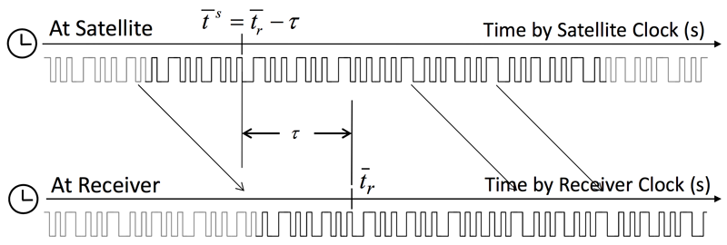 Pseudorange measurement (from the RTKLIB Manual)1
The equation can be written by using the geometric range \(\rho_r^{(s)}\) between satellite and receiver antennas, the receiver and satellite clock biases \(dt_r\) and \(dT^{(s)}\), the ionospheric and tropospheric delays \(I_{r,i}^{(s)}\) and \(T_r^{(s)}\) and the measurement error \(\epsilon_P\) as:
\[\begin{equation} \!\!\!\!\!\! \begin{array}{ccl} P_{r,i}^{(s)} & = & c\left( (t_r+dt_r(t_r)) - (t^{(s)}+dT^{(s)}(t^{(s)})) \right)+ \epsilon_P \\ {} & = & c(t_r - t^{(s)} )+c \left( dt_r(t_r)-dT^{(s)}(t^{(s)}) \right)+\epsilon_P \\ {} & = & \rho_r^{(s)} + c\left( dt_r(t_r) - dT^{(s)}(t^{(s)}) \right) + I_{r,i}^{(s)} + T_r^{(s)} +\epsilon_P ~,\end{array} \end{equation}\]where:
- \(P_{r,i}^{(s)}\) is the pseudorange measurement (in meters).
- \(\rho_{r}^{(s)}\) is the true range from the satellite’s to the receiver’s antenna (in meters).
- \(c\) is the speed of light (in m/s).
- \(dt_r\) is the receiver clock offset from GNSS time (in seconds).
- \(dT^{(s)}\) is the satellite clock offset from GNSS time (in seconds).
- \(I_{r,i}^{(s)}\) is the ionospheric delay (in meters).
- \(T_{r}^{(s)}\) is the tropospheric delay (in meters).
- \(\epsilon_P\) models measurement noise, including satellite orbital errors, receiver’s and satellite’s instrumental delays, effects of multipath propagation and thermal noise (in meters).
GNSS-SDR performs pseudorange generation based on setting a common reception time across all channels2. The result of this approach is not an absolute pseudorange, but a relative pseudorange with respect to the value (of pseudorange) allocated for a reference satellite. This is possible thanks to the time of week (TOW) information, which is the epoch conveyed by the navigation message, and the associated reception time \(t_{r}\), which is the epoch measured by the receiver’s time counter, both available for each satellite.
The first step performed by the common reception time algorithm is the selection of a reference satellite: it is the satellite with the most recent TOW (which is the nearest satellite), denoted as \(\text{TOW}_\text{ref}\), whose associated \(t_{r_\text{ref}}\) is taken as the common reception time for all channels. An initial travel time (\(\tau_\text{ref} = 68.802\) ms is assigned to this satellite, but in general it is a value between \(65\) and \(85\) milliseconds according to the user altitude) that can be easily converted in meters considering the speed of light. Then, the pseudoranges for all other satellites are derived by adding the relative-arrival times. Each travel time \(\tau\) can be computed as:
\[\begin{array}{ccl} \tau^{(s)} & = & \Delta \text{TOW}^{(s)} + \Delta t_r^{(s)} + \tau_\text{ref}\\ & = & \text{TOW}^{(s)} - \text{TOW}_\text{ref} + t_r^{(s)} - t_{r_\text{ref}} + \tau_\text{ref}~, \end{array}\]where \(\Delta \text{TOW}^{(s)}\) is the difference between the reference \(\text{TOW}_\text{ref}\) and the current TOW of the \(s\)-th satellite; \(\Delta t_r^{(s)}\) is the time elapsed between the reference \(t_{r_\text{ref}}\) and the actual receiver time, when the pseudorange must be computed for the specific satellite. This method is equivalent to taking a snapshot of all the channels’ counters at a given time, and thus it can produce pseudoranges at any time, without waiting for a particular bit front on each channel.
The block diagram of such approach is shown below:
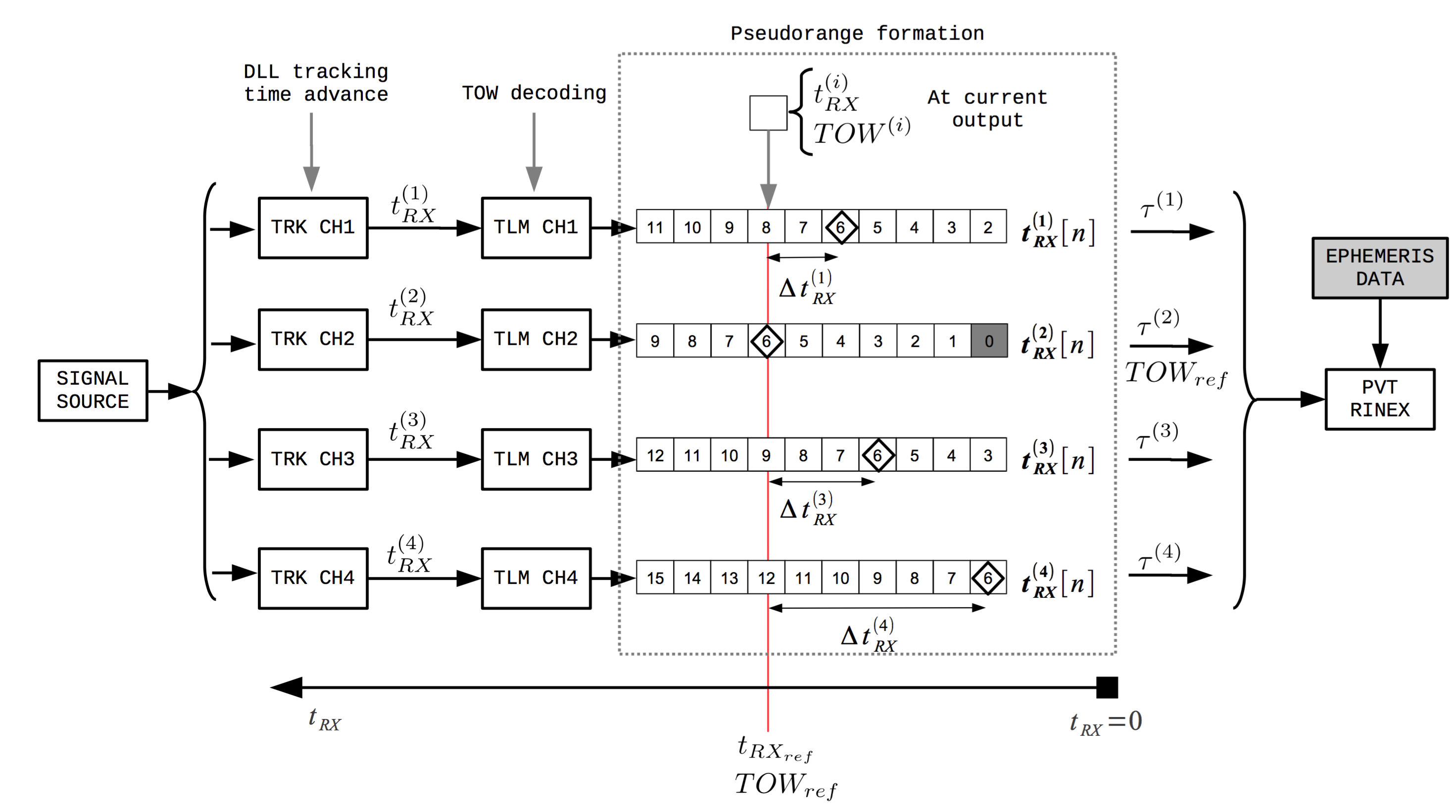 Block diagram of the pseudorange computation using the common reception time approach in GNSS-SDR3
Note that, in the case of a multi-system receiver, all pseudorange observations must be referred to one receiver clock only.
Carrier phase measurement
The carrier phase measurement is actually a measurement of the beat frequency between the received carrier of the satellite signal and a receiver-generated reference frequency. It can be modeled as:
\[\begin{equation} \begin{array}{ccl} \phi_{r,i}^{(s)} & = & \phi_{r,i}(t_r) - \phi_{i}^{(s)}(t^{(s)}) + N_{r,i}^{(s)} + \epsilon_{\phi}\\ {} & = & \left(f_i \left(t_r + dt_r(t_r) - t_0\right) + \phi_{r,0,i}\right)~+\\ {} & {} & - \left(f_i\left(t^{(s)} + dT^{(s)}(t^{(s)}) - t_0 \right) + \phi_{0,i}^{(s)} \right) + N_{r_i}^{(s)} + \epsilon_{\phi}\\ {} & = & \frac{c}{\lambda_i} \left(t_r - t^{(s)}\right) + \frac{c}{\lambda_i}\left(dt_r(t_r) - dT^{(s)}(t^{(s)})\right)~+\\ {} & {} & +~ \phi_{r,0,i} - \phi_{0,i}^{(s)} + N_{r,i}^{(s)} + \epsilon_{\phi}~, \end{array} \end{equation}\]where:
- \(\phi_{r,i}^{(s)}\) is the carrier phase measurement (in cycles) for band \(i\) and satellite \(s\).
- \(\phi_{r,i}(t)\) is the phase for the \(i\)-th band of the receiver’s local oscillator (in cycles) at time \(t\).
- \(\phi_{i}^{(s)}(t)\) is the phase for the \(i\)-th band of the transmitted signal (in cycles) at time \(t\).
- \(t_r\) is the navigation signal reception time at the receiver (in seconds).
- \(t^{(s)}\) is the navigation signal transmission time at the satellite (in seconds).
- \(N_{r,i}^{(s)}\) is the carrier‐phase integer ambiguity (in cycles).
- \(\epsilon_{\phi}\) is a term modeling carrier phase measurement noise, including satellite orbital errors, receiver’s and satellite’s instrumental delays, effects of multipath propagation, and thermal noise (in cycles).
- \(f_i\) is the carrier frequency (in Hz) at band \(i\).
- \(dt_r(t)\) is the receiver clock offset (in seconds) from GPS time at time \(t\).
- \(dT^{(s)}(t)\) is the satellite clock bias (in seconds) from GPS time at time \(t\).
- \(t_0\) is the initial time (in seconds).
- \(\phi_{0,i}^{(s)}\) is the initial phase for the \(i\)-th band of the transmitted signal (in cycles) at time \(t_0\).
- \(c\) is the speed of light (in m/s).
- \(\lambda_i\) is the carrier wavelength (in meters).
As shown in a paper by Petovello and O’Driscoll4, the carrier‐phase integer ambiguity term \(N_{r,i}^{(s)}\) can be written as:
\[N_{r,i}^{(s)} (t_r) = L_{r,i} (t_{r}) - K_{r,i} (t_{r})~,\]where:
- \(L_{r,i} (t_{r})\) is the integer component of the receiver’s numerically controlled oscillator (NCO) phase.
- \(K_{r,i} (t_{r})\) is the integer component of the term \(\left(\frac{\rho_{r}^{(s)}(t_{r})}{\lambda_i} + \phi_{r,0,i} - \phi_{0,i}^{(s)} \right)\).
In order to generate usable phase measurements, the receiver phase observations must maintain a constant integer number of cycles offset from the true carrier phase. That is, if the range increases by one cycle (i.e., one wavelength), the integer component of the NCO, denoted as \(L^{(i)} (t_{r})\), also increments by one cycle.
Phase-range measurement
Phase measurements are sometimes given in meters. This is referred to as phase-range measurement, and it is defined as the carrier phase multiplied by the carrier wavelength \(\lambda_i\). It can be expressed as:
\[\begin{equation} \nonumber \begin{array}{ccl} \Phi_{r,i}^{(s)} & = & \lambda_i \phi_{r,i}^{(s)} \\ {} & = & c\left(t_r - t^{(s)}\right) + c \left(dt_r(t_r) - dT^{(s)}(t^{(s)})\right)~+\\ {} & {} & +~ \lambda_i\left(\phi_{r,0,i} - \phi_{0,i}^{(s)} + N_{r,i}^{(s)}\right) + \lambda_i \epsilon_{\phi}~. \end{array} \end{equation}\]The term \(c(t_r-t^{(s)})\) admits a more detailed model (including antenna phase center offsets and variations, station displacement by earth tides, phase windup effect, and relativity correction on the satellite clock) that will be useful for precise point positioning algorithms. The phase-range measurement can then be modeled as:
\[\begin{eqnarray} \nonumber \Phi_{r,i}^{(s)} & = & \rho_{r}^{(s)} + c\left(dt_r(t_r) - dT^{(s)}(t^{(s)})\right)~+\\ {} & {} & - I_{r,i}^{(s)} + T_{r}^{(s)} + \lambda_i B_{r,i}^{(s)} + d\Phi_{r,i}^{(s)} + \epsilon_{\Phi,i}~, \end{eqnarray}\]where:
- The ionospheric term \(I_{r,i}^{(s)}\) is included with a negative sign due to the phase advancement effect on electromagnetic waves going through a plasmatic media.
- \(B_{r,i}^{(s)} = \phi_{r,0,i} - \phi_{0,i}^{(s)} + N_{r,i}^{(s)}\) is the carrier‐phase bias for the \(i\)-th band (in cycles).
- \(d\Phi_{r,i}^{(s)}\) is a term accounting for satellite’s and receiver’s antenna phase center variation in the \(i\)-th band, defined as:
\(\begin{array}{ccl} d\Phi_{r,i}^{(s)} & = &\mathbf{d}_{r,pco,i}^T \mathbf{e}_{r,enu}^{(s)} + \left(\mathbf{E}^{(s)} \mathbf{d}_{pco,i}^{(s)} \right)^T \mathbf{e}_r^{(s)}~+ \\ {} & {} & +~ d_{r,pcv,i}(El) + d_{pcv,i}^{(s)}(\theta) - \mathbf{d}_{r,disp}^T \mathbf{e}_{r,enu}^{(s)} + \lambda_i \phi_{pw}~, \end{array}\)
where:
- \(\mathbf{d}_{r,pco,i}\) is the receiver’s \(i\)-th band antenna phase center offset in local coordinates (in meters).
- \(d_{r,pcv,i}\) is the receiver’s \(i\)-th band antenna phase center variation (in meters).
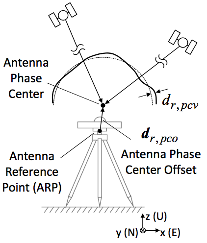
Receiver antenna phase center offset and variation (from the RTKLIB Manual)1
- \(\mathbf{d}_{pco,i}^{(s)}\) is the satellite’s \(i\)-th band antenna phase center offset in satellite body‐fixed coordinates (in meters).
- \(d_{pcv,i}^{(s)}\) is the satellite’s antenna phase center variation (in meters).
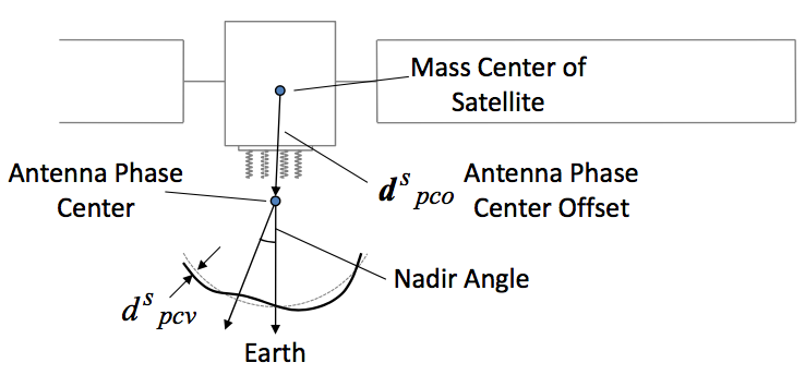
Satellite antenna phase center offset and variation (from the RTKLIB Manual)1
- \(\mathbf{e}_{r,enu}^{(s)}\) is the LOS vector from receiver antenna to satellite in local coordinates.
- \(\mathbf{e}_r^{(s)}\) is the LOS vector from receiver antenna to satellite in ECEF.
- \(\mathbf{E}^{(s)} = \left( {\mathbf{e}_{x}^{(s)}}^T, {\mathbf{e}_{y}^{(s)}}^T, {\mathbf{e}_{z}^{(s)}}^T \right)^T\) is the coordinates transformation matrix from the satellite body‐fixed coordinates to ECEF coordinates, with:
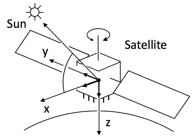
Satellite body-fixed coordinate system (from the RTKLIB Manual)1
- \(\mathbf{r}_{sun}\) is the sun position in ECEF coordinates.
- \(\mathbf{e}^{(s)} = \frac{\mathbf{r}_{sun} - \mathbf{r}^{(s)}}{\left\| \mathbf{r}_{sun} - \mathbf{r}^{(s)}\right\| }\) is a unit vector pointing from satellite \(s\) towards the sun.
- \(\mathbf{e}_{z}^{(s)} = \frac{\mathbf{r}^{(s)}}{\left\| \mathbf{r}^{(s)} \right\|}\) is a unit vector from the satellite to the nadir direction.
- \(\mathbf{e}_{y}^{(s)} = \frac{\mathbf{e}_{z}^{(s)} \times \mathbf{e}^{(s)} }{\left\|\mathbf{e}_{z}^{(s)} \times \mathbf{e}^{(s)} \right\|}\), where \(\times\) denotes the cross-product operator.
- \(\mathbf{e}_{x}^{(s)} = \mathbf{e}_{y}^{(s)} \times \mathbf{e}_{z}^{(s)}\).
- \(\mathbf{d}_{r,disp}\) is the displacement by Earth tides at the receiver position in local coordinates (in meters).
- \(\phi_{pw}\) is the phase wind-up term (in cycles) due to the circular polarization of the GNSS electromagnetic signals. For a receiver with fixed coordinates, the wind-up is due to the satellite orbital motion. As the satellite moves along its orbital path it must perform a rotation to keep its solar panels pointing to the Sun direction in order to obtain the maximum energy while the satellite antenna keeps pointing to the earth’s centre. This rotation causes a phase variation that the receiver misunderstands as a range variation.
- \(\epsilon_{\Phi,i} = \lambda_i \epsilon_{\phi}\) is a term modeling instrumental phase noise.
Doppler shift measurement
The Doppler effect5 (or the Doppler shift) is the change in frequency for an observer (in this case, the GNSS receiver) moving relative to its source (in this case, a given GNSS satellite \(s\)). The relationship between observed frequency \(f\) and emitted frequency \(f_i\) is given by
\[f = \left( \frac{c+v_r}{c+v^{(s)}}\right)f_i~.\]Since the speeds of the receiver \(\mathbf{v}_r(t)\) and the satellite \(\mathbf{v}^{(s)}\) are small compared to the speed of the wave, the difference between the observed frequency \(f\) and emitted frequency \(f_i\) can be approximated by
\[f_{D_{i}}^{(s)} = -f_i\frac{\partial \tau^{(s)}(t)}{\partial t}~.\]Then, the Doppler shift measurement can be written as:
\[\begin{equation} \!\!\!\!\!\!\!\!\!\!\begin{array}{ccl} f_{D_{i}}^{(s)} & = & -f_i \frac{\partial (t_r - t^{(s)}) }{\partial t}\\ {} & = & -f_i \frac{\partial \left( \frac{1}{c} \left(\rho_r^{(s)} + I_{r,i}^{(s)} + T_r^{(s)}\right) + dt_r(t_r) - dT^{(s)}(t^{(s)}) \right)}{\partial t}\\ {} & = & -\frac{f_i}{c}\frac{\partial \left( \left\| \mathbf{r}^{(s)}(t^{(s)}) - \mathbf{r}_r(t_r) \right\| + I_{r,i}^{(s)} + T_{r}^{(s)}+c(dt_r(t_r) - dT^{(s)}(t^{(s)})) \right)}{\partial t}\\ {} & = & -\frac{f_i}{c} \left( \left( \mathbf{v}^{(s)}(t^{(s)}) - \mathbf{v}_{r}(t_r) \right)^T \frac{\left( \mathbf{r}^{(s)}(t^{(s)}) - \mathbf{r}_r(t_r) \right)}{\left\| \mathbf{r}^{(s)}(t^{(s)}) - \mathbf{r}_r(t_r) \right\|} + \frac{\partial I_{r,i}^{(s)}}{\partial t} + \right.\\ {} & {} & \left. +~ \frac{\partial T_{r}^{(s)}}{\partial t} + c\frac{\partial dt_r(t_r)}{\partial t} - c\frac{\partial dT^{(s)}(t^{(s)})}{\partial t} \right)\\ {} & = & -\frac{f_i}{c} \left( \left( \mathbf{v}^{(s)}(t^{(s)}) - \mathbf{v}_{r}(t_r) \right)^T \mathbf{e}_r^{(s)} + c\frac{\partial dt_r(t_r)}{\partial t} - c\frac{\partial dT^{(s)}(t^{(s)})}{\partial t} \right) + \epsilon_{f_{D}}~, \end{array} \end{equation}\]where \(\mathbf{r}_r(t)\) and \(\mathbf{v}_r(t)\) are the position and velocity of the receiver at the instant \(t\). The term \(\left( \mathbf{v}^{(s)}(t^{(s)}) - \mathbf{v}_{r}(t_r) \right)^T \mathbf{e}_r^{(s)}\) is the radial velocity from the receiver relative to the satellite, and \(\frac{\partial dt_r(t_r)}{\partial t}\) and \(\frac{\partial dT^{(s)}(t^{(s)})}{\partial t}\) are the receiver and satellite clocks drift, respectively. The Doppler shift measurement is given in Hz.
Pseudorange rate measurement
Doppler shift measurements are sometimes given in m/s. This is referred to as pseudorange rate measurement, and it is defined as the Doppler shift multiplied by the negative of carrier wavelength \(\lambda_i\). Its model can be written as:
\[\begin{eqnarray} \dot{P}_{r,i}^{(s)} & = & -\lambda_i f_{D_{i}}^{(s)} \nonumber \\ {} & = & \left( \mathbf{v}^{(s)}(t^{(s)}) - \mathbf{v}_{r}(t_r) \right)^T \mathbf{e}_r^{(s)} ~+\\ {} & {} & + c \left( \frac{\partial dt_r(t_r)}{\partial t} - \frac{\partial dT^{(s)}(t^{(s)})}{\partial t}\right) + \epsilon_{\dot{P}}~. \nonumber \end{eqnarray}\]Carrier-smoothing of code pseudoranges
The noisy (but unambiguous) code pseudorange measurements can be smoothed with the precise (but ambiguous) carrier phase measurements. A simple algorithm, known as the Hatch filter, is given as follows6:
Let \(P_{r,i}^{(s)}[n]\) and \(\Phi_{r,i}^{(s)}[n]\) be the code and carrier measurements of a given satellite \(s\), in the band \(i\), at the time \(n\). Thence, the smoothed code \(\hat{P}_{r,i}^{(s)}[n]\) can be computed as:
\[\begin{equation} \label{eq:smoothing} \begin{array}{ccl} \hat{P}_{r,i}^{(s)}[k] & = & \frac{1}{M} P_{r,i}^{(s)}[k] ~+\\ {} & {} & +~ \frac{M-1}{M}\left[ \hat{P}_{r,i}^{(s)}[k-1] \left(\Phi_{r,i}^{(s)}[k] - \Phi_{r,i}^{(s)}[k-1] \right) \right]~, \end{array} \end{equation}\]where \(n=k\) when \(k<M\) and \(n=M\) when \(k \geq M\).
The algorithm is initialized with:
\[\begin{equation} \nonumber \hat{P}_{r,i}^{(s)}[1] = P_{r,i}^{(s)}[1]~. \end{equation}\]This algorithm is initialized every time that a carrier phase cycle-slip occurs.
Implementation: Hybrid_Observables
This implementation computes observables by collecting the outputs of channels for all kinds of allowed GNSS signals. You always can use this implementation in your configuration file, since it accepts all kind of (single- or multi-band, single- or multi-constellation) receiver configurations.
It accepts the following parameters:
| Parameter | Description | Required |
|---|---|---|
implementation |
Hybrid_Observables |
Mandatory |
enable_carrier_smoothing |
[true, false]: If set to true, it enables carrier smoothing of code pseudoranges. It defaults to false. |
Optional |
smoothing_factor |
If enable_carrier_smoothing is set to true, this parameter sets the smoothing factor \(M\) (see equation (\(\ref{eq:smoothing}\))). It defaults to 200. |
Optional |
dump |
[true, false]: If set to true, it enables the Observables internal binary data file logging. Storage in .mat files readable from Matlab, Octave and Python is available starting from GNSS-SDR v0.0.10, see below. It defaults to false. |
Optional |
dump_filename |
If dump is set to true, name of the file in which internal data will be stored. This parameter accepts either a relative or an absolute path; if there are non-existing specified folders, they will be created. It defaults to ./observables.dat |
Optional |
dump_mat |
[true, false]. If dump=true, when the receiver exits it can convert the “.dat” files stored by this block into “.mat” files directly readable from Matlab and Octave. If the receiver has processed more than a few minutes of signal, this conversion can take a long time. In systems with limited resources, you can turn off this conversion by setting this parameter to false. It defaults to true, so “.mat” files are generated by default if dump=true. |
Optional |
Observables implementation: Hybrid_Observables.
Example:
;######### OBSERVABLES CONFIG ############
Observables.implementation=Hybrid_Observables
Observables.dump=false
Binary output
If Observables.dump=true, the logging of data is also delivered in MATLAB
Level 5 MAT-file
v7.3
format, in a file with the same name as dump_filename but terminated in .mat
instead of .dat. This is a compressed binary file format that can be easily
read with Matlab or Octave, by doing load observables.mat, or in Python via
the h5py library. The stored
variables are matrices with a number of rows equal to the total number of
channels set up in the configuration file, and a number of columns equal to the
number of epochs (that is, tracking integration times). This block stores the
following variables:
Carrier_Doppler_hz: Doppler estimation in each channel, in [Hz].Carrier_phase_cycles: Carrier phase estimation in each channel, in [cycles].Flag_valid_pseudorange: Pseudorange computation status in each channel.PRN: Satellite ID processed in each channel.Pseudorange_m: Pseudorange computation in each channel, in [m].RX_time: Receiving time in each channel, in seconds after the start of the week.TOW_at_current_symbol_s: Time of week of the current symbol, in [s].
;######### OBSERVABLES CONFIG ############
Observables.implementation=Hybrid_Observables
Observables.dump=true
References
-
T. Takasu, RTKLIB ver. 2.4.2 Manual. April 29, 2013. ↩ ↩2 ↩3 ↩4
-
M. Petovello, M. Rao, G. Falca, Code Tracking and Pseudoranges: How can pseudorange measurements be generated from code tracking?, Inside GNSS, vol. 7, no. 1, pp. 26–33, Jan./Feb. 2012. ↩
-
J. Arribas, M. Branzanti, C. Fernández-Prades and P. Closas, Fastening GPS and Galileo Tight with a Software Receiver, in Proc. of the 27th International Technical Meeting of The Satellite Division of the Institute of Navigation (ION GNSS+ 2014), Tampa, Florida, Sep. 2014, pp. 1383 - 1395. ↩
-
M. Petovello, C. O’Driscoll, Carrier phase and its measurements for GNSS: What is the carrier phase measurement? How is it generated in GNSS receivers? Inside GNSS, vol. 5, no. 5, pp. 18–22, Jul./Aug. 2010. ↩
-
C. Doppler, Über das farbige Licht der Doppelsterne und einiger anderer Gestirne des Himmels (On the colored light of the double stars and certain other stars of the heavens), Abh. Kniglich Bhmischen Ges. Wiss., vol. 2, pp. 467–482, 1842. ↩
-
M. Petovello, L. Lo Presti, M. Visintin, Can you list all the properties of the carrier-smoothing filter?, Inside GNSS, vol. 10, no. 4, pp. 32–37, Jul./Aug. 2015. ↩