Input Filter
The Input Filter is the second processing block inside a Signal Conditioner
when the latter is using a Signal_Conditioner
implementation.
The role of an Input Filter block is to filter noise and possible interferences from the incoming signal.
There are three kinds of filter implementations available:
- Finite Impulse Response (FIR) filters, implementing a fixed frequency mask
for out-of-band noise or frequency alias suppression.
Fir_Filterfor baseband signals.Freq_Xlating_Fir_Filterfor signals modulated at a given intermediate frequency.
- Adaptive filters for interference mitigation.
Pulse_Blanking_Filterfor pulsed interferences.Notch_Filter,Notch_Filter_Litefor narrowband interferences.
- Short circuit.
Pass_Throughcopy the input samples to the output buffer.
In the presence of noise and interferences, the signal y(t) received at the antenna of a GNSS receiver can be modeled as1
\[\begin{equation} y(t) = x(t) + i(t) + \eta(t)~, \end{equation}\]where:
- \(x(t)\) is the useful signal containing the different GNSS components which will be used for receiver operations,
- \(i(t)\) is the interference signal, and
- \(\eta(t)\) is a noise term usually modeled as a complex circularly symmetric Gaussian random process. The samples are assumed independent and identically distributed.
The sequence \(y[n]\) is obtained by amplifying, down-converting, and digitizing the analog signal \(y(t)\) with a sampling frequency \(f_s\).
Interference Cancellation consists of removing \(i[n]\) from \(y[n]\) by means of a signal processing algorithm. The underlying idea seems straightforward but, in practice, Interference Cancellation becomes a complicated matter due to the huge variety of interference sources that may coexist within the GNSS signal band. For instance, the interference may be pulsed or continuous. In the first case, the period between pulses, time duration, intensity, and bandwidth of the pulses can be constant or vary over time. In the second case, the intensity, instantaneous frequency and frequency rate of the interference may also behave randomly. For this reason, there is no “one-fits-all” algorithm for interference mitigation. Furthermore, during last years research literature has been populated with new signal processing techniques that perform many kinds of Interference Cancellation2.
Finite Impulse Response (FIR) filters
Implementation: Fir_Filter
This implementation, based on the Parks-McClellan algorithm, computes the optimal (in the Chebyshev/minimax sense) FIR filter impulse response given a set of band edges, the desired response on those bands, and the weight given to the error in those bands. The Parks-McClellan algorithm uses the Remez exchange algorithm and Chebyshev approximation theory to design filters with an optimal fit between the desired and actual frequency responses.
This implementation accepts the following parameters:
| Parameter | Description | Required |
|---|---|---|
implementation |
Fir_Filter |
Mandatory |
input_item_type |
[cbyte, cshort, gr_complex]: Input data type. This implementation only accepts streams of complex data types. |
Mandatory |
output_item_type |
[cbyte, cshort, gr_complex]: Output data type. You can use this implementation to upcast the data type (i.e., from cbyte to gr_complex and from cshort to gr_complex). |
Mandatory |
taps_item_type |
[float]: Type and resolution for the taps of the filter. Only float is allowed in the current version. |
Mandatory |
number_of_taps |
Number of taps in the filter. Increasing this parameter increases the processing time. | Mandatory |
number_of_bands |
Number of frequency bands in the filter. | Mandatory |
band1_begin |
Frequency at the band edges [ b1 e1 b2 e2 b3 e3…]. Frequency is in the range [0, 1], with 1 being the Nyquist frequency (\(\frac{F_s}{2}\)). The number of band_begin and band_end elements must match the number of bands. |
Mandatory |
band1_end |
Frequency at the band edges [ b1 e1 b2 e2 b3 e3 …] | Mandatory |
band2_begin |
Frequency at the band edges [ b1 e1 b2 e2 b3 e3 …] | Mandatory |
band2_end |
Frequency at the band edges [ b1 e1 b2 e2 b3 e3 …] | Mandatory |
ampl1_begin |
Desired amplitude at the band edges [ a(b1) a(e1) a(b2) a(e2) …]. The number of ampl_begin and ampl_end elements must match the number of bands. |
Mandatory |
ampl1_end |
Desired amplitude at the band edges [ a(b1) a(e1) a(b2) a(e2) …]. | Mandatory |
ampl2_begin |
Desired amplitude at the band edges [ a(b1) a(e1) a(b2) a(e2) …]. | Mandatory |
ampl2_end |
Desired amplitude at the band edges [ a(b1) a(e1) a(b2) a(e2) …]. | Mandatory |
band1_error |
Weighting applied to band 1 (usually 1). | Mandatory |
band2_error |
Weighting applied to band 2 (usually 1). | Mandatory |
filter_type |
[bandpass, hilbert, differentiator]: type of filter to be used. |
Mandatory |
grid_density |
Determines how accurately the filter will be constructed. The minimum value is 16; higher values make the filter slower to compute, but often results in filters that more exactly match an equiripple filter. | Mandatory |
dump |
[false, true]: Flag for storing the signal at the filter output in a file. It defaults to false. |
Optional |
dump_filename |
If dump is set to true, path to the file where data will be stored. |
Optional |
Input Filter implementation: Fir_Filter.
Possible filter_type are:
-
passband: designs a FIR filter, using the weightsband1_error,band2_error, etc. to weight the fit in each frequency band. -
hilbert: designs linear-phase filters with odd symmetry. This class of filters has the desired amplitude of 1 across the entire band. -
differentiator: For nonzero amplitude bands, it weights the error by a factor of \(1/f\) so that the error at low frequencies is much smaller than at high frequencies. For FIR differentiators, which have an amplitude characteristic proportional to frequency, these filters minimize the maximum relative error (the maximum of the ratio of the error to the desired amplitude).
The following figure shows the relationship between \(f\) = [band1_begin band1_end
band2_begin band2_end] and \(a\) = [ampl1_begin ampl1_end
ampl2_begin ampl2_end] vectors in defining a desired frequency
response for the Input Filter:
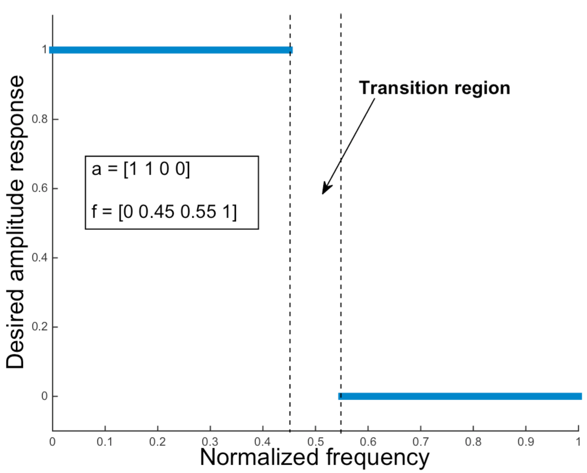 Definition of frequency mask parameters.
If you have access to MATLAB, you can plot easily the frequency response of the filter. Just copy these lines into the command window:
f = [0 0.45 0.55 1];
a = [1 1 0 0];
b = firpm(5, f, a);
[h, w] = freqz(b, 1, 512);
plot(f, a, w/pi, abs(h))
legend('Ideal', 'Filter design')
xlabel('Radian Frequency (\omega/\pi)'), ylabel('Magnitude')
Example of GNSS-SDR configuration:
;######### INPUT_FILTER CONFIG ############
InputFilter.implementation=Fir_Filter

InputFilter.dump=false
InputFilter.dump_filename=./input_filter.dat

InputFilter.input_item_type=cbyte
InputFilter.output_item_type=gr_complex
InputFilter.taps_item_type=float
InputFilter.number_of_taps=5

InputFilter.number_of_bands=2

InputFilter.band1_begin=0.0
InputFilter.band1_end=0.45
InputFilter.band2_begin=0.55
InputFilter.band2_end=1.0

InputFilter.ampl1_begin=1.0
InputFilter.ampl1_end=1.0
InputFilter.ampl2_begin=0.0
InputFilter.ampl2_end=0.0

InputFilter.band1_error=1.0
InputFilter.band2_error=1.0

InputFilter.filter_type=bandpass
InputFilter.grid_density=16
Implementation: Freq_Xlating_Fir_Filter
This implementation features a frequency-translating FIR filter. This is often used when input data is at an intermediate frequency, as it performs filtering, decimation, and frequency shifting in one single step. The basic principle of this block is to perform:
Input signal \(\rightarrow\) Filtering \(\rightarrow\) \(\downarrow N\) \(\rightarrow\) \(\times \exp\{ - j2 \pi \frac{f_{IF}}{f_s} N \}\) \(\rightarrow\) Output signal.
This block is a wrapper of GNU Radio’s freq_xlating_fir_filter_impl.h block. It applies the baseband filter moved up to the intermediate frequency \(f_{IF}\), then it performs decimation by a factor \(N\) and a de-rotation with \(\times \exp\{ -j 2 \pi \frac{f_{IF}}{f_s}N \}\) to downshift the signal to baseband. Thus, the filter parameters apply to the signal before decimation.
The block is ideally suited for a “channel selection filter” and can be efficiently used to select and decimate a narrow band signal out of wide bandwidth input.
This implementation accepts the following parameters:
| Parameter | Description | Required |
|---|---|---|
implementation |
Freq_Xlating_Fir_Filter |
Mandatory |
filter_type |
[lowpass, bandpass, hilbert, differentiator]: type of filter to be used after the frequency translation. |
Mandatory |
input_item_type |
[byte, short, float, gr_complex]: This implementation accepts as input data type real samples. It also accepts complex samples of the type gr_complex, assuming the presence of an intermediate frequency. The filter also works with IF=0. |
Mandatory |
output_item_type |
[cbyte, cshort, gr_complex]: Output data type. You can use this implementation to upcast the data type. |
Mandatory |
sampling_frequency |
Specifies the input sample rate \(f_s\), in samples per second. | Mandatory |
IF |
Specifies the intermediate frequency \(f_{IF}\) to be removed, in Hz. It defaults to \(0\) Hz (i.e., baseband complex signal). | Optional |
decimation_factor |
Decimation factor \(N\) (defaults to 1). Needs to be an integer. | Optional |
taps_item_type |
[float]: Type and resolution for the taps of the filter. Only float is allowed in the current version. |
Mandatory |
number_of_taps |
Number of taps in the filter. Increasing this parameter increases the processing time. If filter_type is set to lowpass, this parameter has no effect |
Optional |
number_of_bands |
Number of frequency bands in the filter. If filter_type is set to lowpass, this parameter has no effect |
Optional |
band1_begin |
Frequency at the band edges [ b1 e1 b2 e2 b3 e3…]. Frequency is in the range [0, 1], with 1 being the Nyquist frequency (\(\frac{F_s}{2}\)). The number of band_begin and band_end elements must match the number of bands. If filter_type is set to lowpass, this parameter has no effect |
Optional |
band1_end |
Frequency at the band edges [ b1 e1 b2 e2 b3 e3 …]. If filter_type is set to lowpass, this parameter has no effect |
Optional |
band2_begin |
Frequency at the band edges [ b1 e1 b2 e2 b3 e3 …]. If filter_type is set to lowpass, this parameter has no effect |
Optional |
band2_end |
Frequency at the band edges [ b1 e1 b2 e2 b3 e3 …]. If filter_type is set to lowpass, this parameter has no effect |
Optional |
ampl1_begin |
Desired amplitude at the band edges [ a(b1) a(e1) a(b2) a(e2) …]. The number of ampl_begin and ampl_end elements must match the number of bands. If filter_type is set to lowpass, this parameter has no effect |
Optional |
ampl1_end |
Desired amplitude at the band edges [ a(b1) a(e1) a(b2) a(e2) …]. If filter_type is set to lowpass, this parameter has no effect |
Optional |
ampl2_begin |
Desired amplitude at the band edges [ a(b1) a(e1) a(b2) a(e2) …]. If filter_type is set to lowpass, this parameter has no effect |
Optional |
ampl2_end |
Desired amplitude at the band edges [ a(b1) a(e1) a(b2) a(e2) …]. If filter_type is set to lowpass, this parameter has no effect |
Optional |
band1_error |
Weighting applied to band 1 (usually 1). If filter_type is set to lowpass, this parameter has no effect |
Optional |
band2_error |
Weighting applied to band 2 (usually 1). If filter_type is set to lowpass, this parameter has no effect |
Optional |
grid_density |
Determines how accurately the filter will be constructed. The minimum value is 16; higher values make the filter slower to compute, but often results in filters that more exactly match an equiripple filter. If filter_type is set to lowpass, this parameter has no effect |
Optional |
bw |
Specifies the cut-off frequency, in Hz, of the low-pass filter used after the Intermediate Frequency removal. If filter_type is not set to lowpass, this parameter has no effect. It defaults to (sampling_frequency/decimation_factor)/2 Hz. |
Optional |
tw |
Specifies the width of the transition band (centered at bw), in Hz, of the low-pass filter used after the Intermediate Frequency removal. If filter_type is not set to lowpass, this parameter has no effect. It defaults to \(\frac{\text{bw}}{10}\) . |
Optional |
dump |
[false, true]: Flag for storing the signal at the filter output in a file. It defaults to false. |
Optional |
dump_filename |
If dump is set to true, path to the file where data will be stored. |
Optional |
Input Filter implementation: Freq_Xlating_Fir_Filter.
Example:
;######### INPUT_FILTER CONFIG ############
InputFilter.implementation=Freq_Xlating_Fir_Filter

InputFilter.dump=false
InputFilter.dump_filename=./input_filter.dat

InputFilter.input_item_type=byte
InputFilter.output_item_type=gr_complex
InputFilter.taps_item_type=float

InputFilter.number_of_taps=5
InputFilter.number_of_bands=2

InputFilter.band1_begin=0.0
InputFilter.band1_end=0.45
InputFilter.band2_begin=0.55
InputFilter.band2_end=1.0

InputFilter.ampl1_begin=1.0
InputFilter.ampl1_end=1.0
InputFilter.ampl2_begin=0.0
InputFilter.ampl2_end=0.0

InputFilter.band1_error=1.0
InputFilter.band2_error=1.0
InputFilter.filter_type=bandpass
InputFilter.grid_density=16

InputFilter.IF=2000000
InputFilter.sampling_frequency=8000000
Adaptive filters for interference mitigation
The first step of any interference mitigation algorithm consists of determining whether the interference is present within the receiver’s frequency band. A simple method is to calculate the input signal power and compare it against a certain threshold. This threshold should be set according to the signal level in absence of the interference signal. Since the power of the GNSS useful signal components at the receiver’s antenna is extremely weak (several tens of dB below the background noise), the input signal power when the interference source is switched off is in practice the same as the background noise power. This is
\[\begin{equation} E \{ | y(t) |^2 \} \approx E \{ | \eta(t) |^2 \} = \sigma^2~. \end{equation}\]After the ADC step and exploiting the statistical properties of \(\eta[n]\) (i.i.d. Gaussian symmetric circular noise), it is possible to guarantee a certain probability of false alarm, i.e. the probability of detecting the interference when the jamming signal is not present. Comparing the signal magnitude against the threshold and taking a decision in all the samples is not feasible in real-time applications, so the detection algorithm runs on signal segments of length \(L\) samples. The energy of a signal segment is
\[\begin{equation} E_s = \sum_{l=1}^{L} | y[l] |^2~. \end{equation}\]The random variable \(\frac{E_s}{\sigma^2}\) follows a chi-squared distribution with \(2L\) degrees of freedom. According to the tabulated values of that distribution, it is possible to set the threshold that produces a given probability of false alarm. When the segment’s energy exceeds the detection threshold, then the segment is processed with the interference mitigation algorithm.
Note that \(\sigma^2\) should be estimated by a noise floor power estimation method. With the purpose of minimizing the random effects, several noise power estimations are averaged on consecutive signal segments. In addition, as the receiver background noise may change along the time, the estimation of \(\sigma^2\) is performed periodically. In this sense, the minimum signal length to be processed (filtered by a mitigation input filter) is one signal segment because the detection of an interference affects to the entire segment. The figure below summarizes the underlying idea.
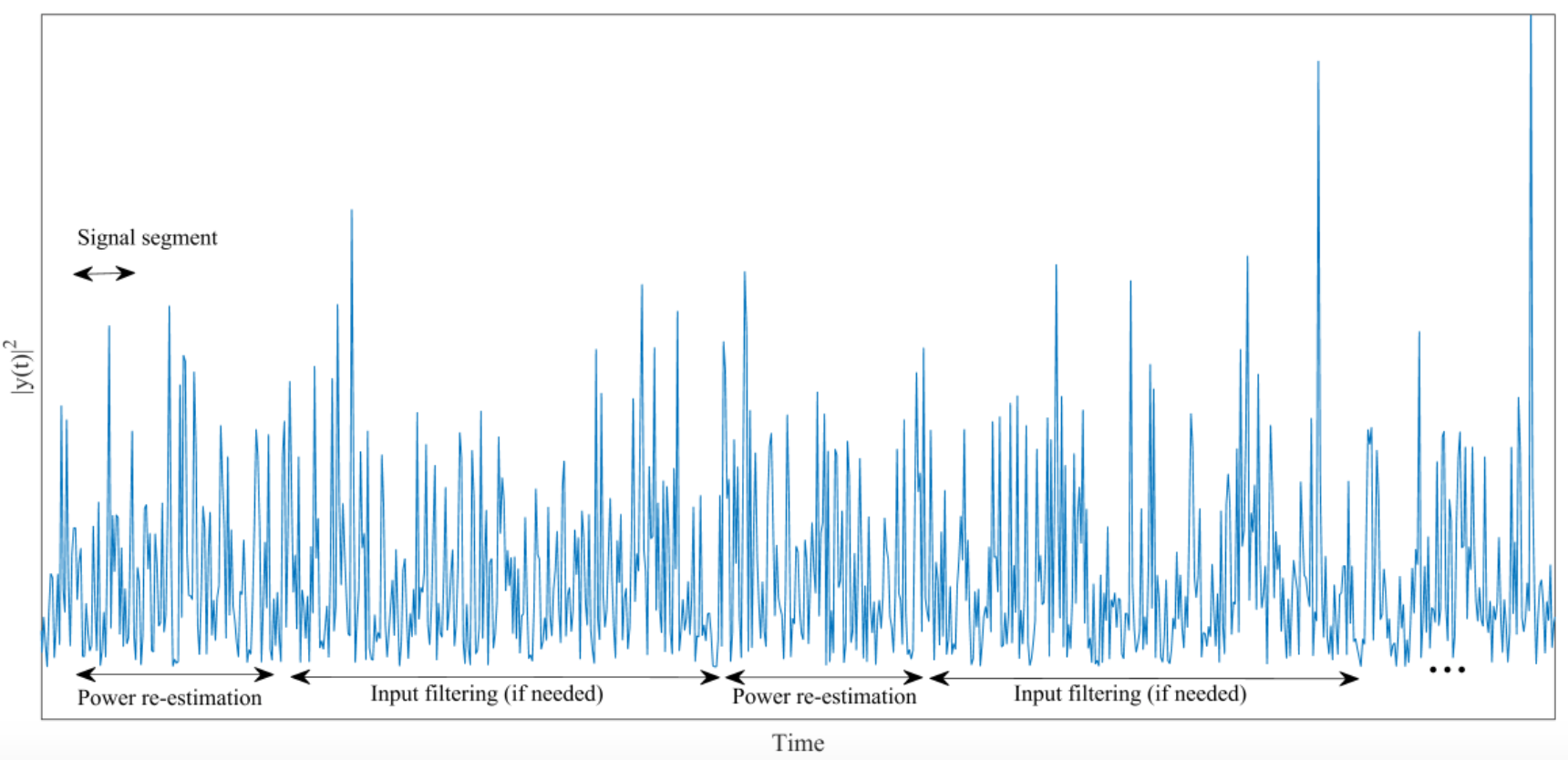 Noise estimation parameters.
Implementation: Pulse_Blanking_Filter
The basic principle of a Pulse Blanking filter is illustrated in the figure below. If the input signal has a squared magnitude within an observation window that is greater than the blanking threshold, \(T_h\), then the output signal is set to zero. Otherwise, the output is equal to the input. Replacing the corrupted samples by zero ensures that correlation values are minimally distorted.
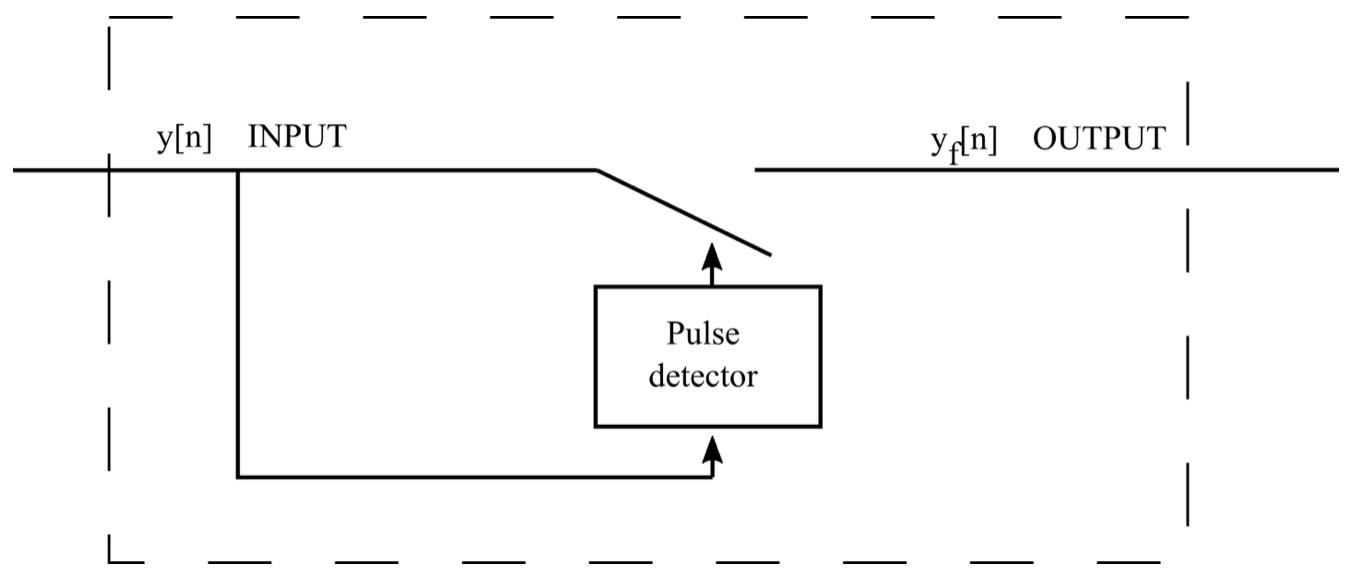 Diagram of the Pulse Blanking filter.
where:
\[\begin{equation} y_f[n] = \left\{ \begin{array}{cl} y[n] & \text{if}\;\; E_s < T_h \\ 0 & \text{if}\;\; E_s > T_h \end{array} \right. \end{equation}\]The implementation of this block provides the following interface:
| Parameter | Description | Required |
|---|---|---|
implementation |
Pulse_Blanking_Filter |
Mandatory |
pfa |
Probability of false alarm. It defaults to \(0.04\) | Optional |
length |
Number of signal samples \(L\) per analysis segment. It defaults to \(32\). | Optional |
item_type |
Data type. This implementation only accepts gr_complex. It defaults to gr_complex. |
Optional |
segments_est |
Number of signal segments in a noise floor estimation epoch. It defaults to \(12500\). | Optional |
segments_reset |
Number of signal segments between two consecutive noise floor estimations. It defaults to \(5000000\). | Optional |
IF |
Specifies the intermediate frequency \(f_{IF}\) to be removed, in Hz. It defaults to \(0\) Hz (i.e., baseband complex signal). | Optional |
sampling_frequency |
If IF is set to any value below or above \(\pm 1\) Hz, sampling_frequency specifies the sample rate \(f_s\), in samples per second. If IF is not set, this parameter has no effect. It defaults to \(f_s = 4000000\) Sps. |
Optional |
bw |
If IF is set to any value below or above \(\pm 1\) Hz, bw specifies the cut-off frequency, in Hz, of the low-pass filter used after the Intermediate Frequency removal. If IF is not set, this parameter has no effect. It defaults to \(2000000\) Hz. |
Optional |
tw |
If IF is set to any value above \(1\) Hz, tw specifies the width of the transition band (centered at bw), in Hz, of the low-pass filter used after the Intermediate Frequency removal. If IF is not set, this parameter has no effect. It defaults to \(\frac{\text{bw}}{10}\). |
Optional |
dump |
[true, false]. Flag for storing the signal at the filter output in a file. It defaults to false. |
Optional |
dump_filename |
If dump is set to true, path to the file where output data is stored. |
Optional |
Input Filter implementation: Pulse_Blanking_Filter.
Example:
;######### INPUT_FILTER CONFIG ############
InputFilter.implementation=Pulse_Blanking_Filter
InputFilter.pfa=0.01
InputFilter.segments_est=5000
Implementation: Notch_Filter
The aim of the Notch filter is to eliminate jamming signals who are instantaneously narrowband and, also, their instantaneous frequency changes over time.
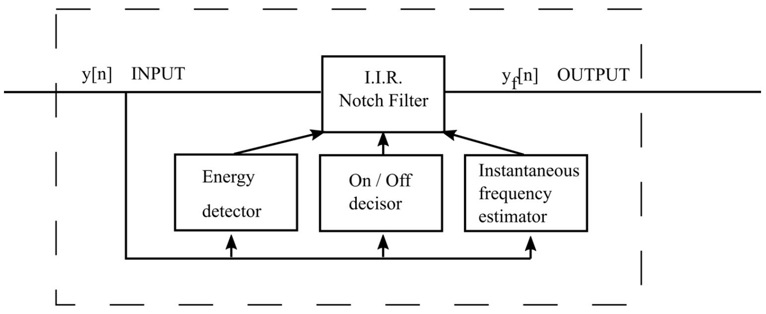 Diagram of the notch filter.
When Interference Cancellation is adopted, the interfering signal is at first removed from \(y[n]\), and subsequent signal processing is applied to \(y_f[n] = y[n] − i[n]\). Since \(i[n]\) is usually not known, an estimation technique is required to reconstruct it and to obtain \(\hat{i}[n]\). This interference \(i[n]\) is usually estimated by considering a specific signal model that depends only on a reduced number of parameters. Let us consider a single component signal1
\[\begin{equation} i[n]=A[n]\exp \{j\varphi[n]\}~, \end{equation}\]where \(A[n]\) and \(\varphi[n]\) are two real signals with \(A[n] \in [0,+\infty)\) and \(\varphi[n]\in(−\pi,\pi]\). Although this model is quite general, the hypothesis assumed by the single component model is that \(i[n]\) is instantaneously narrow band, i.e., it has a single frequency component at each instant in time. Continuous Wave and chirp signals are examples of waveforms that can be described by this model. The instantaneous frequency of a single component signal is defined as the discrete derivative of its phase:
\[\begin{equation} f_i[n] = \frac{1}{2\pi} \left( \varphi[n] - \varphi[n-1] \right)~. \end{equation}\]This block implements a simple, single-sample Prony’s frequency estimator3. The interference frequency is estimated as
\[\begin{equation} \hat{f_i}[n] = \frac{1}{2\pi} \angle \{ y[n] y^{*}[n-1] \}~. \end{equation}\]Single component signals can be generated by a first-order recurrence equation,
\[\begin{equation} i[n] = a[n]i[n−1]~, \end{equation}\]where \(a[n]\) is a time-varying coefficient that can be expressed as:
\[\begin{equation} a[n] = \frac{i[n]}{i[n-1]} = \frac{A[n]}{A[n-1]} \exp \{ j 2 \pi f_i[n] \}~. \end{equation}\]This principle is exploited in a single-pole notch filter which is characterized by the following transfer function:
\[\begin{equation} H_n(z) = \frac{ 1-z_0[n]z^{-1} }{ 1-k_a z_0[n]z^{-1} }~, \end{equation}\]where \(z_0[n]\) is the complex zero of the filter and \(k_a\) is the pole contraction factor, ranging from \(0\) to \(1\). The pole contraction factor determines the bandwidth of the Notch filter, the closer to \(1\), the narrower the filter bandwidth.
The implementation of this block provides the following interface:
| Parameter | Description | Required |
|---|---|---|
implementation |
Notch_Filter |
Mandatory |
p_c_factor |
Pole contraction factor of the filter, \(k_a\). It ranges from \(0\) to \(1\). The higher the value, the lower the filter bandwidth. It defaults to \(0.9\) | Optional |
pfa |
Probability of false alarm. It defaults to \(0.001\) | Optional |
length |
Number of signal samples \(L\) per analysis segment. It defaults to \(32\). | Optional |
item_type |
Data type. This implementation only accepts gr_complex. It defaults to gr_complex. |
Optional |
segments_est |
Number of signal segments in a noise floor estimation epoch. It defaults to \(12500\). | Optional |
segments_reset |
Number of signal segments between two consecutive noise floor estimations. It defaults to \(5000000\). | Optional |
dump |
[true, false]. Flag for storing the signal at the filter output in a file. It defaults to false. |
Optional |
dump_filename |
If dump is set to true, path to the file where output data is stored. |
Optional |
Input Filter implementation: Notch_Filter.
Example:
;######### INPUT_FILTER CONFIG ############
InputFilter.implementation=Notch_Filter
InputFilter.p_c_factor=0.95
InputFilter.segments_est=5000
Implementation: Notch_Filter_Lite
This is an implementation of a notch filter in which the user can choose the updating rate of the filter central frequency estimation. This requires lower computational resources since the Prony estimation is no longer performed sample by sample.
That update rate must be set according to the variation rate of the jammer frequency. Slow variations in the jammer frequency are well tracked by a slow updating rate, but this is not true for fast variations. In this implementation, the maximum updating rate available is one update per signal segment, this is to say, \(\frac{f_s}{L}\), where \(f_s\) is the sampling frequency and \(L\) is the number of samples per signal segment.
The implementation of this block provides the following interface:
| Parameter | Description | Required |
|---|---|---|
implementation |
Notch_Filter_Lite |
Mandatory |
p_c_factor |
Pole contraction factor of the filter, \(k_a\). It ranges from \(0\) to \(1\). The higher the value, the narrower the filter bandwidth. It defaults to \(0.9\) | Optional |
pfa |
Probability of false alarm. It defaults to \(0.001\) | Optional |
coeff_rate |
Updating rate of the filter coefficients. It defaults to tenth the sampling frequency set at SignalSource.sampling_frequency. |
Optional |
length |
Number of signal samples per analysis segment. It defaults to \(32\). | Optional |
item_type |
Data type. This implementation only accepts gr_complex. It defaults to gr_complex. |
Optional |
segments_est |
Number of signal segments in a noise floor estimation epoch. It defaults to \(12500\). | Optional |
segments_reset |
Number of signal segments between two consecutive noise floor estimations. It defaults to \(5000000\). | Optional |
dump |
[true, false]. Flag for storing the signal at the filter output in a file. It defaults to false. |
Optional |
dump_filename |
If dump is set to true, path to the file where output data is stored. |
Optional |
Input Filter implementation: Notch_Filter_Lite.
Example:
;######### INPUT_FILTER CONFIG ############
InputFilter.implementation=Notch_Filter_Lite
InputFilter.p_c_factor=0.95
InputFilter.length=64
Short circuit
Implementation: Pass_Through
This implementation copies samples from its input to its output, without performing any filtering or data type conversion.
It accepts the following parameters:
| Parameter | Description | Required |
|---|---|---|
implementation |
Pass_Through |
Mandatory |
item_type |
[gr_complex, cshort, cbyte]: Format of data samples. It defaults to gr_complex. |
Optional |
Input Filter implementation: Pass_Through.
Examples:
;######### INPUT FILTER CONFIG ############
InputFilter.implementation=Pass_Through
;######### INPUT FILTER CONFIG ############
InputFilter.implementation=Pass_Through
InputFilter.item_type=cshort
References
-
D. Borio, A Multi-State Notch Filter for GNSS Jamming Mitigation, in Proc. of the International Conference on Localization and GNSS (ICL-GNSS), pp. 1-6, June 2014, Helsinki, Finland. DOI: 10.1109/ICL-GNSS.2014.6934175. ↩ ↩2
-
F. Dovis, Ed. GNSS Interference Threats and Countermeasures, Artech House, Noordwood, MA, 2015. ↩
-
R. Prony, Essai expérimental et analytique sur les lois de la dilabilité des fluides élastiques, et sur celles de la force expansive de la vapeur de l’eau et de la vapeur de l’alkool, à différentes températures, Journal de l’École Polytechnique, Floréal et Prairial, Vol. 1, no. 22, pp. 24–76, 1795. ↩
Leave a comment